Skip to main content

Appendix C — Tips and Tricks

Note: This appendix is still under construction as we update some materials from the First Edition to the Second Edition. If you would like to contribute, please check us out on GitHub at https://github.com/moderndive/moderndive_book.

Needed packages

Let’s load all the packages needed for this chapter (this assumes you’ve already installed them). Recall from our discussion in Section 4.4 that loading the tidyverse package by running library(tidyverse) loads the following commonly used data science packages all at once:

• ggplot2 for data visualization
• dplyr for data wrangling
• tidyr for converting data to “tidy” format
• readr for importing spreadsheet data into R
• As well as the more advanced purrr, tibble, stringr, and forcats packages.

If needed, read Section 1.3 for information on how to install and load R packages.

library(tidyverse)
library(scales)
library(janitor)
library(dygraphs)
library(nycflights23)

C.1 Data wrangling

In this Section, we address some of the most common data wrangling questions we’ve encountered in student projects (shout out to Dr. Jenny Smetzer for her work setting this up!):

• Section C.1.1: Dealing with missing values
• Section C.1.2: Reordering bars in a barplot
• Section C.1.3: Showing money on an axis
• Section C.1.4: Changing values inside cells
• Section C.1.5: Converting a numerical variable to a categorical one
• Section C.1.6: Computing proportions
• Section C.1.7: Dealing with %, commas, and $

Cartoon ninja mascot representing the “data wrangling” appendix.

Let’s load an example movies dataset, pare down the rows and columns a bit, and then show the first 10 rows using slice().

movies_ex <- read_csv("https://moderndive.com/data/movies.csv") %>%
  filter(type %in% c("action", "comedy", "drama", "animated", "fantasy", "rom comedy")) %>%
  select(-over200)

movies_ex %>%
  slice(1:10)

# A tibble: 10 × 5
   name             score rating type       millions
   <chr>            <dbl> <chr>  <chr>         <dbl>
 1 2 Fast 2 Furious  48.9 PG-13  action        NA   
 2 A Guy Thing       39.5 PG-13  rom comedy    15.5 
 3 A Man Apart       42.9 R      action        26.2 
 4 A Mighty Wind     79.9 PG-13  comedy        17.8 
 5 Agent Cody Banks  57.9 PG     action        47.8 
 6 Alex & Emma       35.1 PG-13  rom comedy    14.2 
 7 American Wedding  50.7 R      comedy       104.  
 8 Anger Management  62.6 PG-13  comedy       134.  
 9 Anything Else     63.3 R      rom comedy     3.21
10 Bad Boys II       38.1 R      action       138.  

C.1.1 Dealing with missing values

You see the revenue in millions value for the movie “2 Fast 2 Furious” is NA (missing). So the following occurs when computing the median revenue:

movies_ex %>%
  summarize(mean_profit = median(millions))

# A tibble: 1 × 1
  mean_profit
        <dbl>
1          NA

You should always think about why a data value might be missing and what that missingness may mean. For example, imagine you are conducting a study on the effects of smoking on lung cancer and a lot of your patients’ data is missing because they died of lung cancer. If you just “sweep these patients under the rug” and ignore them, you are clearly biasing the results.

While there are statistical methods to deal with missing data they are beyond the reach of this class. The easiest thing to do is to remove all missing cases, but you should always at the very least report to the reader if you do so, as by removing the missing values you may be biasing your results.

You can do this with a na.rm = TRUE argument like so:

movies_ex %>%
  summarize(mean_profit = median(millions, na.rm = TRUE))

# A tibble: 1 × 1
  mean_profit
        <dbl>
1        43.4

If you decide you want to remove the row with the missing data, you can use the filter function like so:

movies_no_missing <- movies_ex %>%
  filter(!is.na(millions))

movies_no_missing %>%
  slice(1:10)

# A tibble: 10 × 5
   name             score rating type       millions
   <chr>            <dbl> <chr>  <chr>         <dbl>
 1 A Guy Thing       39.5 PG-13  rom comedy    15.5 
 2 A Man Apart       42.9 R      action        26.2 
 3 A Mighty Wind     79.9 PG-13  comedy        17.8 
 4 Agent Cody Banks  57.9 PG     action        47.8 
 5 Alex & Emma       35.1 PG-13  rom comedy    14.2 
 6 American Wedding  50.7 R      comedy       104.  
 7 Anger Management  62.6 PG-13  comedy       134.  
 8 Anything Else     63.3 R      rom comedy     3.21
 9 Bad Boys II       38.1 R      action       138.  
10 Bad Santa         75.8 R      comedy        59.5 

We see “2 Fast 2 Furious” is now gone.

C.1.2 Reordering bars in a barplot

Let’s compute the total revenue for each movie type and plot a barplot.

revenue_by_type <- movies_ex %>%
  group_by(type) %>%
  summarize(total_revenue = sum(millions))
revenue_by_type

# A tibble: 6 × 2
  type       total_revenue
  <chr>              <dbl>
1 action               NA 
2 animated            561.
3 comedy             2287.
4 drama               840.
5 fantasy             509.
6 rom comedy          492.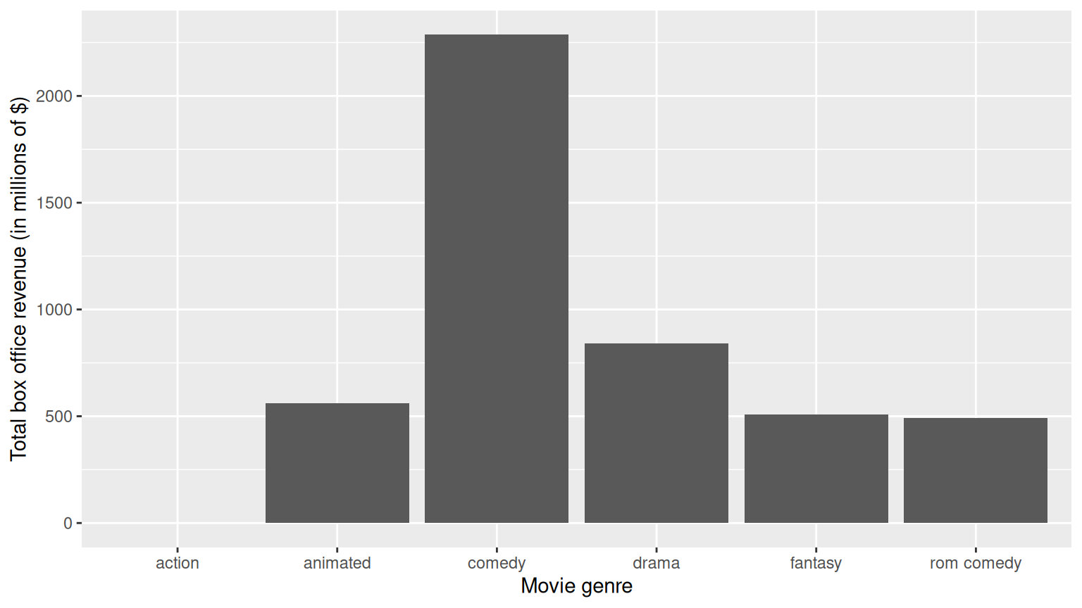

ggplot(revenue_by_type, aes(x = type, y = total_revenue)) +
  geom_col() +
  labs(x = "Movie genre", y = "Total box office revenue (in millions of $)")

Say we want to reorder the categorical variable type so that the bars show in a different order. We can reorder the bars by manually defining the order of the levels in the factor() command:

type_levels <- c("rom comedy", "action", "drama", "animated", "comedy", "fantasy")

revenue_by_type <- revenue_by_type %>%
  mutate(type = factor(type, levels = type_levels))

ggplot(revenue_by_type, aes(x = type, y = total_revenue)) +
  geom_col() +
  labs(x = "Movie genre", y = "Total boxoffice revenue (in millions of $)")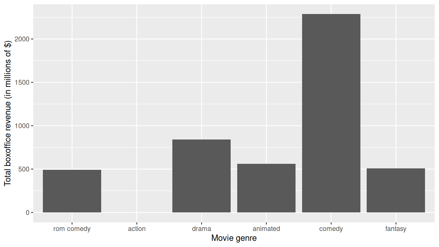

Or if you want to reorder type in ascending order of total_revenue, we use reorder():

revenue_by_type <- revenue_by_type %>%
  mutate(type = reorder(type, total_revenue))

ggplot(revenue_by_type, aes(x = type, y = total_revenue)) +
  geom_col() +
  labs(
    x = "Movie genre", y = "Total boxoffice revenue (in millions of $)"
  )

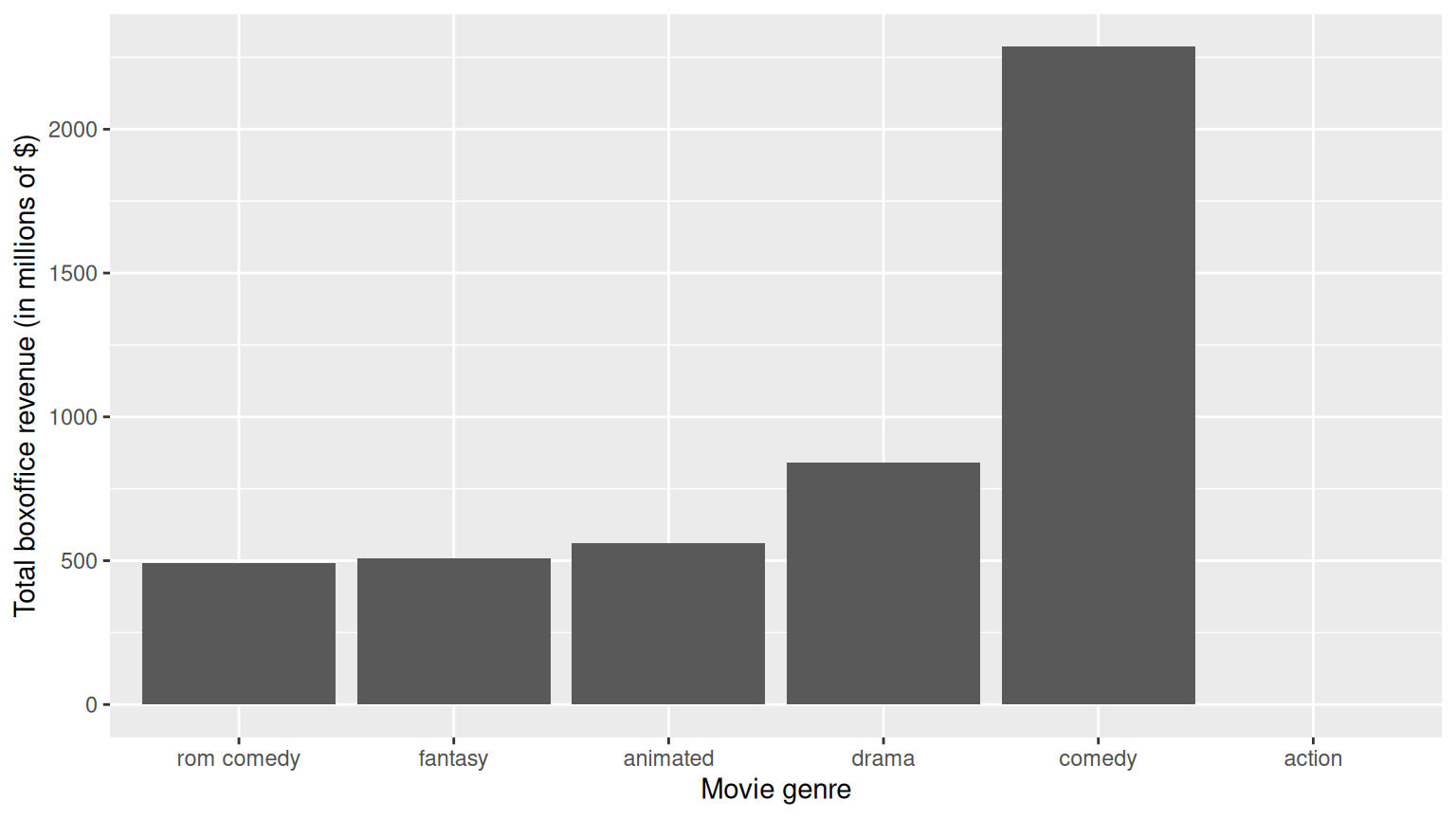
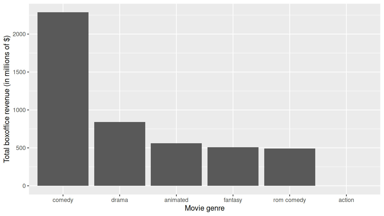
Or if you want to reorder type in descending order of total_revenue, just put a - sign in front of -total_revenue in reorder():

revenue_by_type <- revenue_by_type %>%
  mutate(type = reorder(type, -total_revenue))

ggplot(revenue_by_type, aes(x = type, y = total_revenue)) +
  geom_col() +
  labs(
    x = "Movie genre", y = "Total boxoffice revenue (in millions of $)"
  )

For more advanced categorical variable (i.e. factor) manipulations, check out the forcats package. Note: forcats is an anagram of factors.

Hex logo for the forcats package — a stylized fox above the package name.

C.1.3 Showing money on an axis

movies_ex <- movies_ex %>%
  mutate(revenue = millions * 10^6)

ggplot(data = movies_ex, aes(x = rating, y = revenue)) +
  geom_boxplot() +
  labs(x = "rating", y = "Revenue in $", title = "Profits for different movie ratings")

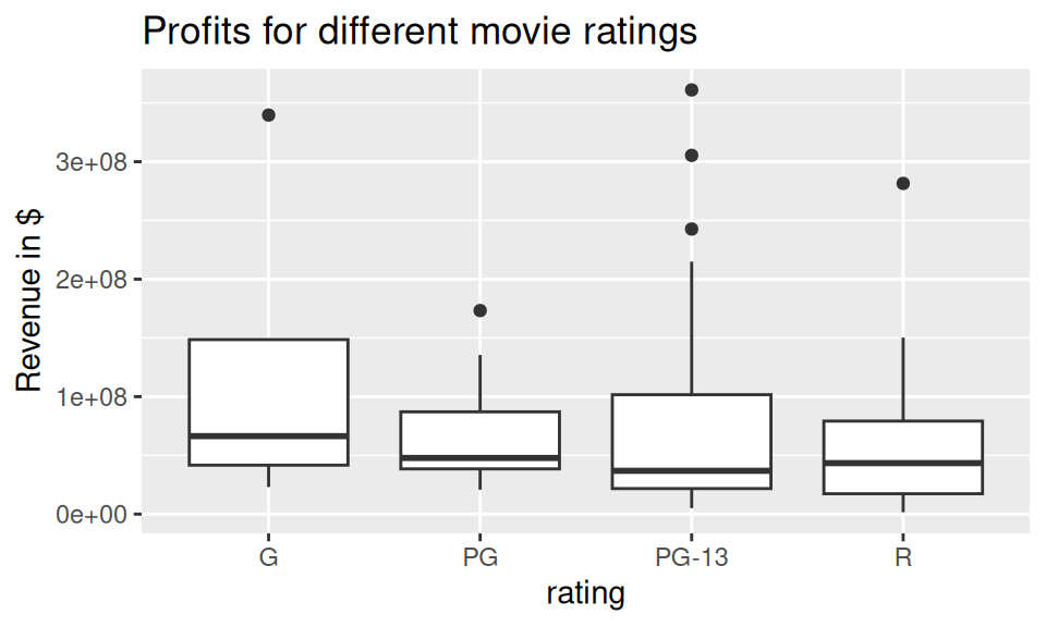
Google “ggplot2 axis scale dollars” and click on the first link and search for the word “dollars”. You’ll find:

# Don't forget to load the scales package first!
library(scales)

ggplot(data = movies_ex, aes(x = rating, y = revenue)) +
  geom_boxplot() +
  labs(x = "rating", y = "Revenue in $", title = "Profits for different movie ratings") +
  scale_y_continuous(labels = dollar)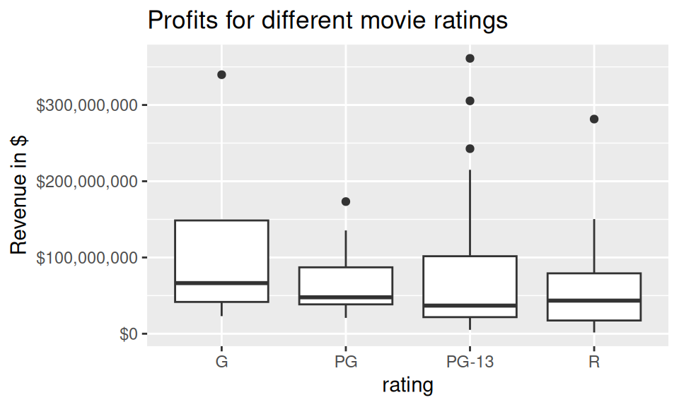

C.1.4 Changing values inside cells

The rename() function in the dplyr package renames column/variable names. To “rename” values inside cells of a particular column, you need to mutate() the column using one of the three functions below. There might be other ones too, but these are the three we’ve seen the most. In these examples, we’ll change values in the variable type.

1. if_else()
2. recode()
3. case_when()

if_else()

Switch all instances of rom comedy with romantic comedy using if_else() from the dplyr package. If a particular row has type == "rom comedy", then return "romantic comedy", else return whatever was originally in type. Save everything in a new variable type_new:

movies_ex %>%
  mutate(type_new = if_else(type == "rom comedy", "romantic comedy", type)) %>%
  slice(1:10)

# A tibble: 10 × 7
   name             score rating type       millions    revenue type_new       
   <chr>            <dbl> <chr>  <chr>         <dbl>      <dbl> <chr>          
 1 2 Fast 2 Furious  48.9 PG-13  action        NA           NA  action         
 2 A Guy Thing       39.5 PG-13  rom comedy    15.5   15545000  romantic comedy
 3 A Man Apart       42.9 R      action        26.2   26247999  action         
 4 A Mighty Wind     79.9 PG-13  comedy        17.8   17781000  comedy         
 5 Agent Cody Banks  57.9 PG     action        47.8   47811001  action         
 6 Alex & Emma       35.1 PG-13  rom comedy    14.2   14219000  romantic comedy
 7 American Wedding  50.7 R      comedy       104.   104441000  comedy         
 8 Anger Management  62.6 PG-13  comedy       134.   134404010  comedy         
 9 Anything Else     63.3 R      rom comedy     3.21   3212000. romantic comedy
10 Bad Boys II       38.1 R      action       138.   138397000  action         

Do the same here, but return "not romantic comedy" if type is not "rom comedy" and this time overwrite the original type variable:

movies_ex %>%
  mutate(type = if_else(type == "rom comedy", "romantic comedy", "not romantic comedy")) %>%
  slice(1:10)

# A tibble: 10 × 6
   name             score rating type                millions    revenue
   <chr>            <dbl> <chr>  <chr>                  <dbl>      <dbl>
 1 2 Fast 2 Furious  48.9 PG-13  not romantic comedy    NA           NA 
 2 A Guy Thing       39.5 PG-13  romantic comedy        15.5   15545000 
 3 A Man Apart       42.9 R      not romantic comedy    26.2   26247999 
 4 A Mighty Wind     79.9 PG-13  not romantic comedy    17.8   17781000 
 5 Agent Cody Banks  57.9 PG     not romantic comedy    47.8   47811001 
 6 Alex & Emma       35.1 PG-13  romantic comedy        14.2   14219000 
 7 American Wedding  50.7 R      not romantic comedy   104.   104441000 
 8 Anger Management  62.6 PG-13  not romantic comedy   134.   134404010 
 9 Anything Else     63.3 R      romantic comedy         3.21   3212000.
10 Bad Boys II       38.1 R      not romantic comedy   138.   138397000 

recode()

if_else() is rather limited however. What if we want to “rename” all type so that they start with uppercase? Use recode():

movies_ex %>%
  mutate(type_new = recode(type,
    "action" = "Action",
    "animated" = "Animated",
    "comedy" = "Comedy",
    "drama" = "Drama",
    "fantasy" = "Fantasy",
    "rom comedy" = "Romantic Comedy"
  )) %>%
  slice(1:10)

# A tibble: 10 × 7
   name             score rating type       millions    revenue type_new       
   <chr>            <dbl> <chr>  <chr>         <dbl>      <dbl> <chr>          
 1 2 Fast 2 Furious  48.9 PG-13  action        NA           NA  Action         
 2 A Guy Thing       39.5 PG-13  rom comedy    15.5   15545000  Romantic Comedy
 3 A Man Apart       42.9 R      action        26.2   26247999  Action         
 4 A Mighty Wind     79.9 PG-13  comedy        17.8   17781000  Comedy         
 5 Agent Cody Banks  57.9 PG     action        47.8   47811001  Action         
 6 Alex & Emma       35.1 PG-13  rom comedy    14.2   14219000  Romantic Comedy
 7 American Wedding  50.7 R      comedy       104.   104441000  Comedy         
 8 Anger Management  62.6 PG-13  comedy       134.   134404010  Comedy         
 9 Anything Else     63.3 R      rom comedy     3.21   3212000. Romantic Comedy
10 Bad Boys II       38.1 R      action       138.   138397000  Action         

case_when()

case_when() is a little trickier, but allows you to evaluate boolean operations using ==, >, >=, &, |, etc:

movies_ex %>%
  mutate(
    type_new =
      case_when(
        type == "action" & millions > 40 ~ "Big budget action",
        type == "rom comedy" & millions < 40 ~ "Small budget romcom",
        # Need this for everything else that aren't the two cases above:
        TRUE ~ "Rest"
      )
  )

# A tibble: 108 × 7
   name             score rating type       millions    revenue type_new        
   <chr>            <dbl> <chr>  <chr>         <dbl>      <dbl> <chr>           
 1 2 Fast 2 Furious  48.9 PG-13  action        NA           NA  Rest            
 2 A Guy Thing       39.5 PG-13  rom comedy    15.5   15545000  Small budget ro…
 3 A Man Apart       42.9 R      action        26.2   26247999  Rest            
 4 A Mighty Wind     79.9 PG-13  comedy        17.8   17781000  Rest            
 5 Agent Cody Banks  57.9 PG     action        47.8   47811001  Big budget acti…
 6 Alex & Emma       35.1 PG-13  rom comedy    14.2   14219000  Small budget ro…
 7 American Wedding  50.7 R      comedy       104.   104441000  Rest            
 8 Anger Management  62.6 PG-13  comedy       134.   134404010  Rest            
 9 Anything Else     63.3 R      rom comedy     3.21   3212000. Small budget ro…
10 Bad Boys II       38.1 R      action       138.   138397000  Big budget acti…
# ℹ 98 more rows

C.1.5 Converting a numerical variable to a categorical one

Sometimes we want to turn a numerical, continuous variable into a categorical variable. For instance, what if we wanted to have a variable that tells us if a movie made one hundred million dollars or more. That is to say, we can create a binary variable, which is the same thing as a categorical variable with 2 levels. We can again use the mutate() function:

movies_ex %>%
  mutate(big_budget = millions > 100) %>%
  slice(1:10)

# A tibble: 10 × 7
   name             score rating type       millions    revenue big_budget
   <chr>            <dbl> <chr>  <chr>         <dbl>      <dbl> <lgl>     
 1 2 Fast 2 Furious  48.9 PG-13  action        NA           NA  NA        
 2 A Guy Thing       39.5 PG-13  rom comedy    15.5   15545000  FALSE     
 3 A Man Apart       42.9 R      action        26.2   26247999  FALSE     
 4 A Mighty Wind     79.9 PG-13  comedy        17.8   17781000  FALSE     
 5 Agent Cody Banks  57.9 PG     action        47.8   47811001  FALSE     
 6 Alex & Emma       35.1 PG-13  rom comedy    14.2   14219000  FALSE     
 7 American Wedding  50.7 R      comedy       104.   104441000  TRUE      
 8 Anger Management  62.6 PG-13  comedy       134.   134404010  TRUE      
 9 Anything Else     63.3 R      rom comedy     3.21   3212000. FALSE     
10 Bad Boys II       38.1 R      action       138.   138397000  TRUE      

What if you want to convert a numerical variable into a categorical variable with more than 2 levels? One way is to use the cut() command. For instance, below, we cut() the score variable, to recode it into 4 categories:

1. 0 - 40 = bad
2. 40.1 - 60 = so-so
3. 60.1 - 80 = good
4. 80.1+ = great

We set the breaking points for cutting the numerical variable with the c(0, 40, 60, 80, 100) part, and set the labels for each of these bins with the labels = c("bad", "so-so", "good", "great") part. All this action happens inside the mutate() command, so the new categorical variable score_categ is added to the data frame.

movies_ex %>%
  mutate(score_categ = cut(score,
    breaks = c(0, 40, 60, 80, 100),
    labels = c("bad", "so-so", "good", "great")
  )) %>%
  slice(1:10)

# A tibble: 10 × 7
   name             score rating type       millions    revenue score_categ
   <chr>            <dbl> <chr>  <chr>         <dbl>      <dbl> <fct>      
 1 2 Fast 2 Furious  48.9 PG-13  action        NA           NA  so-so      
 2 A Guy Thing       39.5 PG-13  rom comedy    15.5   15545000  bad        
 3 A Man Apart       42.9 R      action        26.2   26247999  so-so      
 4 A Mighty Wind     79.9 PG-13  comedy        17.8   17781000  good       
 5 Agent Cody Banks  57.9 PG     action        47.8   47811001  so-so      
 6 Alex & Emma       35.1 PG-13  rom comedy    14.2   14219000  bad        
 7 American Wedding  50.7 R      comedy       104.   104441000  so-so      
 8 Anger Management  62.6 PG-13  comedy       134.   134404010  good       
 9 Anything Else     63.3 R      rom comedy     3.21   3212000. good       
10 Bad Boys II       38.1 R      action       138.   138397000  bad        

Other options with the cut function:

• By default, if the value is exactly the upper bound of an interval, it’s included in the lessor category (e.g. 60.0 is ‘so-so’ not ‘good’), to flip this, include the argument right = FALSE.
• You could also have R equally divide the variable into a balanced number of groups. For example, specifying breaks = 3 would create 3 groups with approximately the same number of values in each group.

C.1.6 Computing proportions

By using a group_by() followed not by a summarize() as is often the case, but rather a mutate(). So say we compute the total revenue millions for each movie rating and type:

rating_by_type_millions <- movies_ex %>%
  group_by(rating, type) %>%
  summarize(millions = sum(millions)) %>%
  arrange(rating, type)

rating_by_type_millions

# A tibble: 15 × 3
# Groups:   rating [4]
   rating type       millions
   <chr>  <chr>         <dbl>
 1 G      animated      496. 
 2 PG     action         47.8
 3 PG     animated       65.7
 4 PG     comedy        830. 
 5 PG     drama         161. 
 6 PG     fantasy       147. 
 7 PG-13  action         NA  
 8 PG-13  comedy       1208. 
 9 PG-13  drama         306. 
10 PG-13  fantasy       361. 
11 PG-13  rom comedy    406. 
12 R      action       1045. 
13 R      comedy        249. 
14 R      drama         373. 
15 R      rom comedy     86.0

Say within each movie rating (G, PG, PG-13, R), we want to know the proportion of total_millions that made by each movie type (animated, action, comedy, etc). We can:

rating_by_type_millions %>%
  group_by(rating) %>%
  mutate(
    # Compute a new column of the sum of millions split by rating:
    total_millions = sum(millions),
    # Compute the proportion within each rating:
    prop = millions / total_millions
  )

# A tibble: 15 × 5
# Groups:   rating [4]
   rating type       millions total_millions    prop
   <chr>  <chr>         <dbl>          <dbl>   <dbl>
 1 G      animated      496.            496.  1     
 2 PG     action         47.8          1251.  0.0382
 3 PG     animated       65.7          1251.  0.0525
 4 PG     comedy        830.           1251.  0.663 
 5 PG     drama         161.           1251.  0.129 
 6 PG     fantasy       147.           1251.  0.118 
 7 PG-13  action         NA              NA  NA     
 8 PG-13  comedy       1208.             NA  NA     
 9 PG-13  drama         306.             NA  NA     
10 PG-13  fantasy       361.             NA  NA     
11 PG-13  rom comedy    406.             NA  NA     
12 R      action       1045.           1753.  0.596 
13 R      comedy        249.           1753.  0.142 
14 R      drama         373.           1753.  0.213 
15 R      rom comedy     86.0          1753.  0.0491

So for example, the 4 proportions corresponding to R rated movies are 0.596 + 0.142 + 0.213 + 0.0491 = 1.

C.1.7 Dealing with %, commas, and $

Say you have numerical data that are recorded as percentages, have commas, or are in dollar form and hence are character strings. How do you convert these to numerical values? Using the parse_number() function from the readr package inside a mutate()! Shout out to Stack Overflow.

library(readr)
parse_number("10.5%")

[1] 10.5

parse_number("145,897")

[1] 145897

parse_number("$1,234.5")

[1] 1234.5

What about the other way around? Use the scales package!

library(scales)
percent(0.105)

[1] "10%"

comma(145897)

[1] "145,897"

dollar(1234.5)

[1] "$1,234.50"

---

Congratulations. You are now an R Ninja!

Cartoon R ninja mascot celebrating completion of the data-wrangling appendix.

---

C.2 Interactive graphics

C.2.1 Interactive linegraphs

Another useful tool for viewing linegraphs such as this is the dygraph function in the dygraphs package in combination with the dyRangeSelector function. This allows us to zoom in on a selected range and get an interactive plot for us to work with:

library(dygraphs)
library(nycflights23)
flights_day <- mutate(flights, date = as.Date(time_hour))
flights_summarized <- flights_day %>%
  group_by(date) %>%
  summarize(median_arr_delay = median(arr_delay, na.rm = TRUE)) %>%
  as.data.frame()
rownames(flights_summarized) <- flights_summarized$date
flights_summarized <- select(flights_summarized, -date)
dyRangeSelector(dygraph(flights_summarized))

The syntax here is a little different than what we have covered so far. The dygraph function is expecting for the dates to be given as the rownames of the object. We convert our data to a data frame (since tibbles don’t allow for easy row name manipulation), and then remove the date variable from the flights_summarized data frame since it is accounted for in the rownames. Lastly, we run the dygraph function on the new data frame that only contains the median arrival delay as a column and then provide the ability to have a selector to zoom in on the interactive plot via dyRangeSelector. (Note that this plot will only be interactive in the HTML version of this book.)