
3 Data Wrangling
- Chain a sequence of data transformations together using the pipe operator
|> - Apply each of the six core
dplyrverbs to transform a data frame:filter(),select(),mutate(),arrange(),summarize(), andgroup_by() - Combine information from two data frames using the
*_join()family - Recognize when missing values (
NA) require anna.rm = TRUEargument
So far in our journey, we’ve seen how to look at data saved in data frames using the glimpse() and View() functions in Chapter 1, and how to create data visualizations using the ggplot2 package in Chapter 2. In particular, we studied what we term the “five named graphs” (5NG):
- scatterplots via
geom_point() - linegraphs via
geom_line() - boxplots via
geom_boxplot() - histograms via
geom_histogram() - barplots via
geom_bar()orgeom_col()
We created these visualizations using the grammar of graphics, which maps variables in a data frame to the aesthetic attributes of one of the 5 geometric objects. We can also control other aesthetic attributes of the geometric objects such as the size and color as seen in the Gapminder data example in Figure 2.1.
In this chapter, we’ll introduce a series of functions from the dplyr package for data wrangling that will allow you to take a data frame and “wrangle” it (transform it) to suit your needs. Such functions include:
-
filter()a data frame’s existing rows to only pick out a subset of them. For example, theenvoy_flightsdata frame. -
summarize()one or more of its columns/variables with a summary statistic. Examples of summary statistics include the median and interquartile range of temperatures as we saw in Section 2.7 on boxplots. -
group_by()its rows. In other words, assign different rows to be part of the same group. We can then combinegroup_by()withsummarize()to report summary statistics for each group separately. For example, say you don’t want a single overall average departure delaydep_delayfor all threeoriginairports combined, but rather three separate average departure delays, one computed for each of the threeoriginairports. -
mutate()its existing columns/variables to create new ones. For example, convert hourly temperature readings from Fahrenheit to Celsius. -
arrange()its rows. For example, sort the rows ofweatherin ascending or descending order oftemp. -
join()it with another data frame by matching along a “key” variable. In other words, merge these two data frames together.
Notice how we used computer_code font to describe the actions we want to take on our data frames. This is because the dplyr package for data wrangling has intuitively verb-named functions that are easy to remember.
There is a further benefit to learning to use the dplyr package for data wrangling: its similarity to the database querying language SQL (pronounced “sequel” or spelled out as “S-Q-L”). SQL (which stands for “Structured Query Language”) is used to manage large databases quickly and efficiently and is widely used by many institutions with a lot of data. While SQL is a topic left for a book or a course on database management, keep in mind that once you learn dplyr, you can learn SQL easily. We’ll talk more about their similarities in Section 3.7.4.
Needed packages
Let’s load all the packages needed for this chapter (this assumes you’ve already installed them). If needed, read Section 1.3 for information on how to install and load R packages.
3.1 The pipe operator: |>
Before we start data wrangling, let’s first introduce a nifty tool that has been a part of R since May 2021: the native pipe operator |>. The pipe operator allows us to combine multiple operations in R into a single sequential chain of actions. In modern R, the native pipe operator |> is now the default for chaining functions, replacing the previously common tidyverse pipe (%>%) that was loaded with the dplyr package. Introduced in R 4.1.0 in May 2021, |> offers a more intuitive and readable syntax for data wrangling and other tasks, eliminating the need for additional package dependencies.
You’ll still often see R code using %>% in older scripts or searches online, but we’ll use |> in this book. The tidyverse pipe still works, so don’t worry if you see it in other code.
Let’s start with a hypothetical example. Say you would like to perform a hypothetical sequence of operations on a hypothetical data frame x using hypothetical functions f(), g(), and h():
- Take
xthen - Use
xas an input to a functionf()then - Use the output of
f(x)as an input to a functiong()then - Use the output of
g(f(x))as an input to a functionh()
One way to achieve this sequence of operations is by using nesting parentheses as follows:
h(g(f(x)))This code isn’t so hard to read since we are applying only three functions: f(), then g(), then h() and each of the functions is short in its name. Further, each of these functions also only has one argument. However, you can imagine that this will get progressively harder to read as the number of functions applied in your sequence increases and the arguments in each function increase as well. This is where the pipe operator |> comes in handy. |> takes the output of one function and then “pipes” it to be the input of the next function. Furthermore, a helpful trick is to read |> as “then” or “and then.” For example, you can obtain the same output as the hypothetical sequence of functions as follows:
x |>
  f() |>
  g() |>
  h()
You would read this sequence as:
- Take
xthen - Use this output as the input to the next function
f()then - Use this output as the input to the next function
g()then - Use this output as the input to the next function
h()
So while both approaches achieve the same goal, the latter is much more human-readable because you can clearly read the sequence of operations line-by-line. But what are the hypothetical x, f(), g(), and h()? Throughout this chapter on data wrangling:
- The starting value
xwill be a data frame. For example, theflightsdata frame we explored in Section 1.4. - The sequence of functions, here
f(),g(), andh(), will mostly be a sequence of any number of the six data-wrangling verb-named functions we listed in the introduction to this chapter. For example, thefilter(carrier == "MQ")function and argument specified we previewed earlier. - The result will be the transformed/modified data frame that you want. In our example, we’ll save the result in a new data frame by using the
<-assignment operator with the nameenvoy_flightsviaenvoy_flights <-.
envoy_flights <- flights |>
filter(carrier == "MQ")Much like when adding layers to a ggplot() using the + sign, you form a single chain of data wrangling operations by combining verb-named functions into a single sequence using the pipe operator |>. Furthermore, much like how the + sign has to come at the end of lines when constructing plots, the pipe operator |> has to come at the end of lines as well.
Keep in mind, there are many more advanced data-wrangling functions than just the six listed in the introduction to this chapter; you’ll see some examples of these in Section 3.8. However, just with these six verb-named functions you’ll be able to perform a broad array of data-wrangling tasks for the rest of this book.
3.2 filter rows
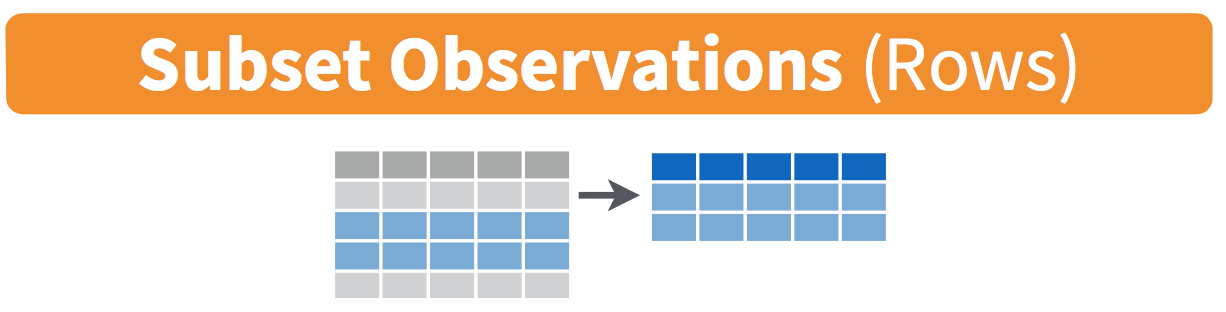
The filter() function here works much like the “Filter” option in Microsoft Excel; it allows you to specify criteria about the values of a variable in your dataset and then filters out only the rows that match that criteria.
We begin by focusing only on flights from New York City to Phoenix, Arizona. The dest destination code (or airport code) for Phoenix, Arizona is "PHX". Run the following and look at the results in RStudio’s spreadsheet viewer to ensure that only flights heading to Phoenix are chosen here:
Note the order of the code. First, take the flights data frame flights then filter() the data frame so that only those where the dest equals "PHX" are included. We test for equality using the double equal sign == and not a single equal sign =. In other words, filter(dest = "PHX") will yield an error. This is a convention across many programming languages. If you are new to coding, you’ll probably forget to use the double equal sign == a few times before you get the hang of it.
You can use other operators beyond just the == operator that tests for equality:
-
>corresponds to “greater than” -
<corresponds to “less than” -
>=corresponds to “greater than or equal to” -
<=corresponds to “less than or equal to” -
!=corresponds to “not equal to.” The!is used in many programming languages to indicate “not.”
Furthermore, you can combine multiple criteria using operators that make comparisons:
-
|corresponds to “or” -
&corresponds to “and”
To see many of these in action, let’s filter flights for all rows that departed from JFK and were heading to Burlington, Vermont ("BTV") or Seattle, Washington ("SEA") and departed in the months of October, November, or December. Run the following:
Note that even though colloquially speaking one might say “all flights heading to Burlington, Vermont and Seattle, Washington,” in terms of computer operations, we really mean “all flights heading to Burlington, Vermont or heading to Seattle, Washington.” For a given row in the data, dest can be "BTV", or "SEA", or something else, but not both "BTV" and "SEA" at the same time. Furthermore, note the careful use of parentheses around dest == "BTV" | dest == "SEA".
We can often skip the use of & and just separate our conditions with a comma. The previous code will return the identical output btv_sea_flights_fall as the following code:
Let’s present another example that uses the ! “not” operator to pick rows that don’t match a criteria. As mentioned earlier, the ! can be read as “not.” Here we are filtering rows corresponding to flights that didn’t go to Burlington, VT or Seattle, WA.
Again, note the careful use of parentheses around the (dest == "BTV" | dest == "SEA"). If we didn’t use parentheses as follows:
flights |> filter(!dest == "BTV" | dest == "SEA")We would be returning all flights not headed to "BTV" or those headed to "SEA", which is an entirely different resulting data frame.
Now say we have a larger number of airports we want to filter for, say "SEA", "SFO", "PHX", "BTV", and "BDL". We could continue to use the | (or) operator.
many_airports <- flights |>
  filter(dest == "SEA" | dest == "SFO" | dest == "PHX" |
         dest == "BTV" | dest == "BDL")
As we progressively include more airports, this will get unwieldy to write. A slightly shorter approach uses the %in% operator along with the c() function. Recall from Section 1.2.1 that the c() function “combines” or “concatenates” values into a single vector of values.
What this code is doing is filtering flights for all flights where dest is in the vector of airports c("BTV", "SEA", "PHX", "SFO", "BDL"). Both outputs of many_airports are the same, but as you can see the latter takes much less energy to code. The %in% operator is useful for looking for matches commonly in one vector/variable compared to another.
As a final note, we recommend that filter() should often be among the first verbs you consider applying to your data. This cleans your dataset to only those rows you care about, or put differently, it narrows down the scope of your data frame to just the observations you care about.
Learning Check
(LC3.1) What’s another way of using the “not” operator ! to filter only the rows that are not going to Burlington, VT nor Seattle, WA in the flights data frame? Test this out using the previous code.
3.3 summarize variables
The next common task when working with data frames is to compute summary statistics. Summary statistics are single numerical values that summarize a large number of values. Commonly known examples of summary statistics include the mean (also called the average) and the median (the middle value). Other examples of summary statistics that might not immediately come to mind include the sum, the smallest value also called the minimum, the largest value also called the maximum, and the standard deviation.
See Appendix A online for a glossary of such summary statistics.
Let’s calculate two summary statistics of the wind_speed variable in the weather data frame: the mean and standard deviation (recall from Section 1.4 that the weather data frame is included in the nycflights23 package). To compute these summary statistics, we need the mean() and sd() summary functions in R. Summary functions in R take in many values and return a single value, as shown in Figure 3.2.

More precisely, we’ll use the mean() and sd() summary functions within the summarize() function from the dplyr package. Note you can also use the British English spelling of summarise(). As shown in Figure 3.3, the summarize() function takes in a data frame and returns a data frame with only one row corresponding to the summary statistics.

We’ll save the results in a new data frame called summary_windspeed that will have two columns/variables: the mean and the std_dev:
# A tibble: 1 × 2
   mean std_dev
  <dbl>   <dbl>
1 NA NAWhy are the values returned NA? NA is how R encodes missing values where NA indicates “not available” or “not applicable.” If a value for a particular row and a particular column does not exist, NA is stored instead. Values can be missing for many reasons. Perhaps the data was collected but someone forgot to enter it. Perhaps the data was not collected at all because it was too difficult to do so. Perhaps there was an erroneous value that someone entered that has been corrected to read as missing. You’ll often encounter issues with missing values when working with real data.
Going back to our summary_windspeed output, by default any time you try to calculate a summary statistic of a variable that has one or more NA missing values in R, NA is returned. To work around this fact, you can set the na.rm argument to TRUE, where rm is short for “remove”; this will ignore any NA missing values and only return the summary value for all non-missing values.
Don’t add na.rm = TRUE reflexively. It silently drops missing values from the calculation, which may not be what you want. Before reaching for na.rm = TRUE, ask: why are these values missing? Were they not collected? Was there a measurement failure? An honest analysis often requires reporting the count of missing values alongside the summary, not just hiding them.
The code that follows computes the mean and standard deviation of all non-missing values of wind_speed:
# A tibble: 1 × 2
   mean std_dev
  <dbl>   <dbl>
1  9.43    5.27
Notice how the na.rm = TRUE are used as arguments to the mean() and sd() summary functions individually, and not to the summarize() function.
However, one needs to be cautious whenever ignoring missing values as we’ve just done. In the upcoming Learning checks questions, we’ll consider the possible ramifications of blindly sweeping rows with missing values “under the rug.” This is in fact why the na.rm argument to any summary statistic function in R is set to FALSE by default. In other words, R does not ignore rows with missing values by default. R is alerting you to the presence of missing data and you should be mindful of this missingness and any potential causes of this missingness throughout your analysis.
What are other summary functions we can use inside the summarize() verb to compute summary statistics? As seen in the diagram in Figure 3.2, you can use any function in R that takes many values and returns just one. Here are just a few:
-
mean(): the average -
sd(): the standard deviation, which is a measure of spread -
min()andmax(): the minimum and maximum values, respectively -
IQR(): interquartile range -
sum(): the total amount when adding multiple numbers -
n(): a count of the number of rows in each group. This particular summary function will make more sense whengroup_by()is covered in Section 3.4.
Learning Check
(LC3.2) Say a doctor is studying the effect of smoking on lung cancer for a large number of patients who have records measured at five-year intervals. She notices that a large number of patients have missing data points because the patient has died, so she chooses to ignore these patients in her analysis. What is wrong with this doctor’s approach?
That introduces survivorship bias / informative dropout. Missingness is not at random (death is related to smoking/cancer). Excluding them biases effects toward healthier survivors and underestimates harm.
(LC3.3) Modify the earlier summarize() function code that creates the summary_windspeed data frame to also use the n() summary function: summarize(... , count = n()). What does the returned value correspond to?
(LC3.4) Why doesn’t the following code work? Run the code line-by-line instead of all at once, and then look at the data. In other words, select and then run summary_windspeed <- weather |> summarize(mean = mean(wind_speed, na.rm = TRUE)) first.
Solution: After the first summarize() you have a 1-row data frame with only mean; wind_speed no longer exists, so the second summarize(sd(wind_speed)) errors. Compute both in one step to fix it:
3.4 group_by rows
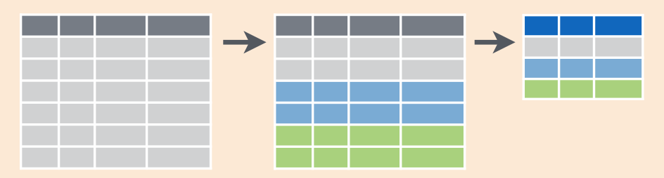
Recall our code from earlier that computed the average wind speed and its spread, keeping the na.rm = TRUE set just in case any missing values are stored in the wind_speed column:
# A tibble: 1 × 2
   mean std_dev
  <dbl>   <dbl>
1  9.43    5.27
Say instead of a single mean wind speed for the whole year, we would like 12 mean wind speeds, one for each of the 12 months separately. In other words, we would like to compute the mean wind speed split by month as shown via generic diagram in Figure 3.4. We can do this by “grouping” wind speed observations by the values of another variable, in this case by the 12 values of the variable month:
# A tibble: 12 × 3
   month  mean std_dev
   <int> <dbl>   <dbl>
 1     1 10.3     6.01
 2     2 10.9     6.60
 3     3 12.4     6.36
 4     4 10.0     5.02
 5     5  8.88    4.45
 6     6  8.52    4.42
 7     7  7.96    4.36
 8     8  8.83    4.34
 9     9  8.92    4.66
10    10  8.21    4.71
11    11  9.48    4.81
12    12  8.77    5.03
This code is identical to the previous code that created summary_windspeed, but with an extra group_by(month) added before the summarize(). Grouping the weather dataset by month and then applying the summarize() functions yields a data frame that displays the mean and standard deviation wind speed split by the 12 months of the year.
It is important to note that the group_by() function doesn’t change data frames by itself. Rather it changes the meta-data, or data about the data, specifically the grouping structure. Only after applying the summarize() function does the data frame change.
As another example, consider the diamonds data frame included in the ggplot2 package:
diamonds# A tibble: 53,940 × 10
carat cut color clarity depth table price x y z
<dbl> <ord> <ord> <ord> <dbl> <dbl> <int> <dbl> <dbl> <dbl>
1 0.23 Ideal E SI2 61.5 55 326 3.95 3.98 2.43
2 0.21 Premium E SI1 59.8 61 326 3.89 3.84 2.31
3 0.23 Good E VS1 56.9 65 327 4.05 4.07 2.31
4 0.29 Premium I VS2 62.4 58 334 4.2 4.23 2.63
5 0.31 Good J SI2 63.3 58 335 4.34 4.35 2.75
6 0.24 Very Good J VVS2 62.8 57 336 3.94 3.96 2.48
7 0.24 Very Good I VVS1 62.3 57 336 3.95 3.98 2.47
8 0.26 Very Good H SI1 61.9 55 337 4.07 4.11 2.53
9 0.22 Fair E VS2 65.1 61 337 3.87 3.78 2.49
10 0.23 Very Good H VS1 59.4 61 338 4 4.05 2.39
# ℹ 53,930 more rowsObserve that the first line of the output reads # A tibble: 53,940 x 10. This is an example of meta-data, in this case the number of observations/rows and variables/columns in diamonds. The actual data itself are the subsequent table of values. Now let’s pipe the diamonds data frame into group_by(cut):
diamonds |>
group_by(cut)# A tibble: 53,940 × 10
# Groups: cut [5]
carat cut color clarity depth table price x y z
<dbl> <ord> <ord> <ord> <dbl> <dbl> <int> <dbl> <dbl> <dbl>
1 0.23 Ideal E SI2 61.5 55 326 3.95 3.98 2.43
2 0.21 Premium E SI1 59.8 61 326 3.89 3.84 2.31
3 0.23 Good E VS1 56.9 65 327 4.05 4.07 2.31
4 0.29 Premium I VS2 62.4 58 334 4.2 4.23 2.63
5 0.31 Good J SI2 63.3 58 335 4.34 4.35 2.75
6 0.24 Very Good J VVS2 62.8 57 336 3.94 3.96 2.48
7 0.24 Very Good I VVS1 62.3 57 336 3.95 3.98 2.47
8 0.26 Very Good H SI1 61.9 55 337 4.07 4.11 2.53
9 0.22 Fair E VS2 65.1 61 337 3.87 3.78 2.49
10 0.23 Very Good H VS1 59.4 61 338 4 4.05 2.39
# ℹ 53,930 more rowsObserve that now there is additional meta-data: # Groups: cut [5] indicating that the grouping structure meta-data has been set based on the 5 possible levels of the categorical variable cut: "Fair", "Good", "Very Good", "Premium", and "Ideal". On the other hand, observe that the data has not changed: it is still a table of 53,940 \(\times\) 10 values. Only by combining a group_by() with another data-wrangling operation, in this case summarize(), will the data actually be transformed.
# A tibble: 5 × 2
cut avg_price
<ord> <dbl>
1 Fair 4359.
2 Good 3929.
3 Very Good 3982.
4 Premium 4584.
5 Ideal 3458.If you would like to remove this grouping structure meta-data, we can pipe the resulting data frame into the ungroup() function:
# A tibble: 53,940 × 10
   carat cut       color clarity depth table price     x     y     z
   <dbl> <ord>     <ord> <ord>   <dbl> <dbl> <int> <dbl> <dbl> <dbl>
 1  0.23 Ideal     E     SI2      61.5    55   326  3.95  3.98  2.43
 2  0.21 Premium   E     SI1      59.8    61   326  3.89  3.84  2.31
 3  0.23 Good      E     VS1      56.9    65   327  4.05  4.07  2.31
 4  0.29 Premium   I     VS2      62.4    58   334  4.2   4.23  2.63
 5  0.31 Good      J     SI2      63.3    58   335  4.34  4.35  2.75
 6  0.24 Very Good J     VVS2     62.8    57   336  3.94  3.96  2.48
 7  0.24 Very Good I     VVS1     62.3    57   336  3.95  3.98  2.47
 8  0.26 Very Good H     SI1      61.9    55   337  4.07  4.11  2.53
 9  0.22 Fair      E     VS2      65.1    61   337  3.87  3.78  2.49
10  0.23 Very Good H     VS1      59.4    61   338  4     4.05  2.39
# ℹ 53,930 more rows
Observe how the # Groups: cut [5] meta-data is no longer present.
Let’s now revisit the n() counting summary function we briefly introduced previously. Recall that the n() function counts rows. This is opposed to the sum() summary function that returns the sum of a numerical variable. For example, suppose we’d like to count how many flights departed each of the three airports in New York City:
# A tibble: 3 × 2
  origin  count
  <chr>   <int>
1 EWR    138578
2 JFK    133048
3 LGA    163726
We see that LaGuardia ("LGA") had the most flights departing in 2023 followed by Newark ("EWR") and lastly by "JFK". Note there is a subtle but important difference between sum() and n(); while sum() returns the sum of a numerical variable, n() returns a count of the number of rows/observations.
Grouping by more than one variable
You are not limited to grouping by one variable. Say you want to know the number of flights leaving each of the three New York City airports for each month. We can also group by a second variable month using group_by(origin, month):
`summarise()` has regrouped the output.
ℹ Summaries were computed grouped by origin and month.
ℹ Output is grouped by origin.
ℹ Use `summarise(.groups = "drop_last")` to silence this message.
ℹ Use `summarise(.by = c(origin, month))` for per-operation grouping
  (`?dplyr::dplyr_by`) instead.
Note that an additional message appears here specifying the grouping done. The .groups argument to summarize() has four options: drop_last, drop, keep, and rowwise:
-
drop_lastdrops the last grouping variable, -
dropdrops all grouping variables, -
keepkeeps all grouping variables, and -
rowwiseturns each row into a group.
In most circumstances, the default is drop_last which drops the last grouping variable. The message is informing us that the default behavior is to drop the last grouping variable, which in this case is month.
by_origin_monthly# A tibble: 36 × 3
# Groups: origin [3]
origin month count
<chr> <int> <int>
1 EWR 1 11623
2 EWR 2 10991
3 EWR 3 12593
4 EWR 4 12022
5 EWR 5 12371
6 EWR 6 11339
7 EWR 7 11646
8 EWR 8 11561
9 EWR 9 11373
10 EWR 10 11805
# ℹ 26 more rowsObserve that there are 36 rows to by_origin_monthly because there are 12 months for 3 airports (EWR, JFK, and LGA). Why do we group_by(origin, month) and not group_by(origin) and then group_by(month)? Let’s investigate:
# A tibble: 12 × 2
   month count
   <int> <int>
 1     1 36020
 2     2 34761
 3     3 39514
 4     4 37476
 5     5 38710
 6     6 35921
 7     7 36211
 8     8 36765
 9     9 35505
10    10 36586
11    11 34521
12    12 33362
What happened here is that the second group_by(month) overwrote the grouping structure meta-data of the earlier group_by(origin), so that in the end we are only grouping by month. The lesson here is if you want to group_by() two or more variables, you should include all the variables at the same time in the same group_by() adding a comma between the variable names.
Learning Check
(LC3.5) Recall from Chapter 2 when we looked at wind speeds by months in NYC. What does the standard deviation column in the summary_monthly_windspeed data frame tell us about wind speeds in NYC throughout the year?
| month | mean | std_dev |
|---|---|---|
| 1 | 10.32 | 6.01 |
| 2 | 10.87 | 6.60 |
| 3 | 12.35 | 6.36 |
| 4 | 10.01 | 5.02 |
| 5 | 8.88 | 4.45 |
| 6 | 8.52 | 4.42 |
| 7 | 7.96 | 4.36 |
| 8 | 8.83 | 4.34 |
| 9 | 8.92 | 4.66 |
| 10 | 8.21 | 4.71 |
| 11 | 9.48 | 4.81 |
| 12 | 8.77 | 5.03 |
Solution: The SD shows within-month variability of wind speeds. The largest spread for a given month was in February with the second highest in March. This would lead us to expect different wind speeds on different days in those months compared to summer months like June, July, and August that have the smallest standard deviations.
(LC3.6) What code would be required to get the mean and standard deviation wind speed for each day in 2023 for NYC?
# A tibble: 364 × 5
    year month   day mean_ws sd_ws
   <int> <int> <int>   <dbl> <dbl>
 1  2023     1     1    8.39  4.57
 2  2023     1     2    5.45  2.50
 3  2023     1     3    4.76  3.29
 4  2023     1     4    5.31  2.84
 5  2023     1     5    5.58  2.94
 6  2023     1     6    6.25  3.77
 7  2023     1     7   10.9   2.82
 8  2023     1     8    8.34  3.38
 9  2023     1     9    8.26  4.20
10  2023     1    10    8.49  2.54
# ℹ 354 more rows
Note: group_by(day) is not enough, because day is a value between 1-31. We need to group_by(year, month, day).
(LC3.7) Recreate by_monthly_origin, but instead of grouping via group_by(origin, month), group variables in a different order group_by(month, origin). What differs in the resulting dataset?
`summarise()` has regrouped the output.
ℹ Summaries were computed grouped by month and origin.
ℹ Output is grouped by month.
ℹ Use `summarise(.groups = "drop_last")` to silence this message.
ℹ Use `summarise(.by = c(month, origin))` for per-operation grouping
(`?dplyr::dplyr_by`) instead.by_monthly_origin| month | origin | count |
|---|---|---|
| 1 | EWR | 11623 |
| 1 | JFK | 10918 |
| 1 | LGA | 13479 |
| 2 | EWR | 10991 |
| 2 | JFK | 10567 |
| 2 | LGA | 13203 |
| 3 | EWR | 12593 |
| 3 | JFK | 12158 |
| 3 | LGA | 14763 |
| 4 | EWR | 12022 |
| 4 | JFK | 11638 |
| 4 | LGA | 13816 |
| 5 | EWR | 12371 |
| 5 | JFK | 11822 |
| 5 | LGA | 14517 |
| 6 | EWR | 11339 |
| 6 | JFK | 11014 |
| 6 | LGA | 13568 |
| 7 | EWR | 11646 |
| 7 | JFK | 11188 |
| 7 | LGA | 13377 |
| 8 | EWR | 11561 |
| 8 | JFK | 11130 |
| 8 | LGA | 14074 |
| 9 | EWR | 11373 |
| 9 | JFK | 10760 |
| 9 | LGA | 13372 |
| 10 | EWR | 11805 |
| 10 | JFK | 10920 |
| 10 | LGA | 13861 |
| 11 | EWR | 10737 |
| 11 | JFK | 10520 |
| 11 | LGA | 13264 |
| 12 | EWR | 10517 |
| 12 | JFK | 10413 |
| 12 | LGA | 12432 |
In by_monthly_origin the month column is now first and the rows are sorted by month instead of origin. If you compare the values of count in by_origin_monthly and by_monthly_origin using the View() function, you’ll see that the values are actually the same, just presented in a different order.
Solution: The counts are identical; only the grouping structure and column order of the grouping keys in the result differ (and potentially the default post-summarize grouping retained/dropped message).
(LC3.8) How could we identify how many flights left each of the three airports for each carrier?
count_flights_by_airport| origin | carrier | num |
|---|---|---|
| EWR | UA | 72545 |
| EWR | YX | 29077 |
| EWR | NK | 9430 |
| EWR | AA | 7559 |
| EWR | B6 | 6855 |
| EWR | DL | 6355 |
| EWR | AS | 3676 |
| EWR | 9E | 1728 |
| EWR | G4 | 671 |
| EWR | MQ | 357 |
| EWR | OO | 325 |
| JFK | B6 | 43418 |
| JFK | DL | 29424 |
| JFK | 9E | 19316 |
| JFK | YX | 17436 |
| JFK | AA | 14319 |
| JFK | OO | 4602 |
| JFK | AS | 4167 |
| JFK | HA | 366 |
| LGA | YX | 42272 |
| LGA | 9E | 33097 |
| LGA | DL | 25783 |
| LGA | AA | 18647 |
| LGA | B6 | 15896 |
| LGA | WN | 12385 |
| LGA | UA | 7096 |
| LGA | NK | 5759 |
| LGA | OO | 1505 |
| LGA | F9 | 1286 |
Note: the n() function counts rows, whereas the sum(VARIABLE_NAME) function sums all values of a certain numerical variable VARIABLE_NAME.
(LC3.9) How does the filter() operation differ from a group_by() followed by a summarize()?
filter() keeps/discards rows based on conditions (no aggregation). group_by()+summarize() collapses rows into group-level statistics.
3.5 mutate existing variables
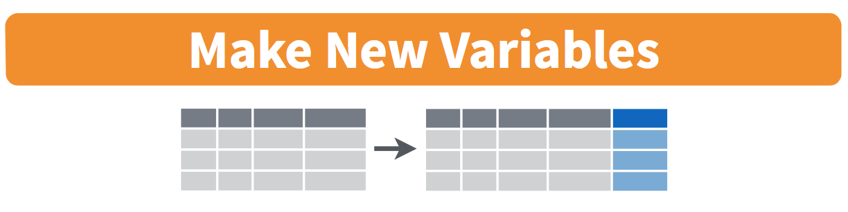
Another common transformation of data is to create/compute new variables based on existing ones as shown in Figure 3.5. For example, say you are more comfortable thinking of temperature in degrees Celsius (°C) instead of degrees Fahrenheit (°F). The formula to convert temperatures from °F to °C is
\[ \text{temp in C} = \frac{\text{temp in F} - 32}{1.8} \]
We can apply this formula to the temp variable using the mutate() function from the dplyr package, which takes existing variables and mutates them to create new ones.
weather <- weather |>
  mutate(temp_in_C = (temp - 32) / 1.8)
In this code, we mutate() the weather data frame by creating a new variable
temp_in_C = (temp - 32) / 1.8,
and then we overwrite the original weather data frame. Why did we overwrite the data frame weather, instead of assigning the result to a new data frame like weather_new?
As a rough rule of thumb, as long as you are not losing original information that you might need later, it’s acceptable practice to overwrite existing data frames with updated ones, as we did here. On the other hand, why did we not overwrite the variable temp, but instead created a new variable called temp_in_C? Because if we did this, we would have erased the original information contained in temp of temperatures in Fahrenheit that may still be valuable to us.
Let’s now compute monthly average temperatures in both °F and °C using the group_by() and summarize() code we saw in Section 3.4:
# A tibble: 12 × 3
   month mean_temp_in_F mean_temp_in_C
   <int>          <dbl>          <dbl>
 1     1           42.8           6.02
 2     2           40.3           4.62
 3     3           43.9           6.61
 4     4           56.0          13.3
 5     5           62.4          16.9
 6     6           69.6          20.9
 7     7           79.2          26.2
 8     8           75.3          24.1
 9     9           70.1          21.2
10    10           61.0          16.1
11    11           47.0           8.31
12    12           43.9           6.62
Let’s consider another example. Passengers are often frustrated when their flight departs late, but aren’t as annoyed if, in the end, pilots can make up some time during the flight. This is known in the airline industry as gain, and we will create this variable using the mutate() function:
flights <- flights |>
mutate(gain = dep_delay - arr_delay)Let’s take a look at only the dep_delay, arr_delay, and the resulting gain variables for the first 5 rows in our updated flights data frame in Table 3.1.
| dep_delay | arr_delay | gain |
|---|---|---|
| 203 | 205 | -2 |
| 78 | 53 | 25 |
| 47 | 34 | 13 |
| 173 | 166 | 7 |
| 228 | 211 | 17 |
The flight in the first row departed 203 minutes late but arrived 205 minutes late, so its “gained time in the air” is a gain of -2 minutes, hence its gain is \(203 - 205 = -2\), which is a loss of 2 minutes. On the other hand, the flight in the third row departed late (dep_delay of 47) but arrived 34 minutes late (arr_delay of 34), so its “gained time in the air” is \(47 - 34 = 13\) minutes, hence its gain is 13.
Let’s look at some summary statistics of the gain variable by considering multiple summary functions at once in the same summarize() code:
gain_summary <- flights |>
  summarize(
    min = min(gain, na.rm = TRUE),
    q1 = quantile(gain, 0.25, na.rm = TRUE),
    median = quantile(gain, 0.5, na.rm = TRUE),
    q3 = quantile(gain, 0.75, na.rm = TRUE),
    max = max(gain, na.rm = TRUE),
    mean = mean(gain, na.rm = TRUE),
    sd = sd(gain, na.rm = TRUE),
    missing = sum(is.na(gain))
  )
gain_summary
# A tibble: 1 × 8
min q1 median q3 max mean sd missing
<dbl> <dbl> <dbl> <dbl> <dbl> <dbl> <dbl> <int>
1 -321 1 11 20 101 9.35 18.4 12534We see for example that the median gain is 11 minutes, while the largest is +101 minutes and the largest negative gain (or loss) at -321 minutes! However, this code would take some time to type out in practice. We’ll see later on in Section 5.1.1 that there is a much more succinct way to compute a variety of common summary statistics: using the tidy_summary() function from the moderndive package.
Recall from Section 2.5 that since gain is a numerical variable, we can visualize its distribution using a histogram.
ggplot(data = flights, mapping = aes(x = gain)) +
  geom_histogram(color = "white", bins = 20)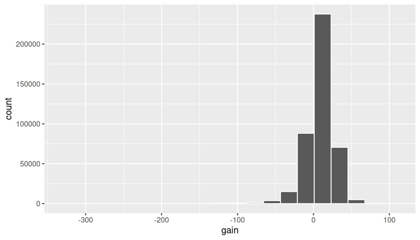
The resulting histogram in Figure 3.6 provides additional perspective on the gain variable than the summary statistics we computed earlier. For example, note that most values of gain are right around 0.
To close out our discussion on the mutate() function to create new variables, note that we can create multiple new variables at once in the same mutate() code. Furthermore, within the same mutate() code we can refer to new variables we just created. As an example, consider the mutate() code Hadley Wickham and Garrett Grolemund show in Chapter 5 of R for Data Science (Grolemund and Wickham 2017):
flights <- flights |>
  mutate(
    gain = dep_delay - arr_delay,
    hours = air_time / 60,
    gain_per_hour = gain / hours
  )
Learning Check
(LC3.10) What do positive values of the gain variable in flights correspond to? What about negative values? And what about a zero value?
gain = dep_delay - arr_delay. Positive ⇒ made up time (arrived earlier/less late than departure delay). Negative ⇒ lost time (arrived even later relative to departure delay). Zero ⇒ no change.
- Say a flight departed 20 minutes late, i.e.
dep_delay = 20. - Then arrived 10 minutes late, i.e.
arr_delay = 10. - Then
gain = dep_delay - arr_delay = 20 - 10 = 10is positive, so it “made up/gained time in the air.” - 0 means the departure and arrival time were the same, so no time was made up in the air. We see in most cases that the
gainis near 0 minutes. - I never understood this. If the pilot says “we’re going make up time in the air” because of delay by flying faster, why don’t you always just fly faster to begin with?
(LC3.11) Could we create the dep_delay and arr_delay columns by simply subtracting dep_time from sched_dep_time and similarly for arrivals? Try the code out and explain any differences between the result and what actually appears in flights.
Not reliably. dep_time/sched_dep_time are clock times (hhmm) and can cross midnight; simple subtraction ignores rollovers/time parsing. The provided dep_delay/arr_delay already account for that logic. You can’t do direct arithmetic on times. The difference in time between 12:03 and 11:59 is 4 minutes, but 1203-1159 = 44.
(LC3.12) What can we say about the distribution of gain? Describe it in a few sentences using the plot and the gain_summary data frame values.
The histogram is centered near 0 with most flights having small gains/losses, and long tails in both directions. Median is near 0 at 11; a few flights gain or lose a lot of minutes, but that’s uncommon.
3.6 arrange and sort rows
One of the most commonly performed data-wrangling tasks is to sort a data frame’s rows in the alphanumeric order of one of the variables. The dplyr package’s arrange() function allows us to sort/reorder a data frame’s rows according to the values of the specified variable.
Suppose we are interested in determining the most frequent destination airports for all domestic flights departing from New York City in 2023:
# A tibble: 118 × 2
   dest  num_flights
   <chr>       <int>
 1 ABQ           228
 2 ACK           916
 3 AGS            20
 4 ALB          1581
 5 ANC            95
 6 ATL         17570
 7 AUS          4848
 8 AVL          1617
 9 AVP           145
10 BDL           701
# ℹ 108 more rows
Observe that by default the rows of the resulting freq_dest data frame are sorted in alphabetical order of destination. Say instead we would like to see the same data, but sorted from the most to the least number of flights (num_flights) instead:
freq_dest |>
  arrange(num_flights)
# A tibble: 118 × 2
dest num_flights
<chr> <int>
1 LEX 1
2 AGS 20
3 OGG 20
4 SBN 24
5 HDN 28
6 PNS 71
7 MTJ 77
8 ANC 95
9 VPS 109
10 AVP 145
# ℹ 108 more rowsThis is, however, the opposite of what we want. The rows are sorted with the least frequent destination airports displayed first. This is because arrange() always returns rows sorted in ascending order by default. To switch the ordering to be in “descending” order instead, we use the desc() function as so:
# A tibble: 118 × 2
   dest  num_flights
   <chr>       <int>
 1 BOS         19036
 2 ORD         18200
 3 MCO         17756
 4 ATL         17570
 5 MIA         16076
 6 LAX         15968
 7 FLL         14239
 8 CLT         12866
 9 DFW         11675
10 SFO         11651
# ℹ 108 more rows
3.7 join data frames
Another common data transformation task is “joining” or “merging” two different datasets. For example, in the flights data frame, the variable carrier lists the carrier code for the different flights. While the corresponding airline names for "UA" and "AA" might be somewhat easy to guess (United and American Airlines), what airlines have codes "G4", "HA", and "B6"? This information is provided in a separate data frame airlines.
View(airlines)We see that in airlines, carrier is the carrier code, while name is the full name of the airline company. Using this table, we can see that "G4", "HA", and "B6" correspond to Allegiant Air, Hawaiian Airlines, and JetBlue, respectively. However, wouldn’t it be nice to have all this information in a single data frame instead of two separate data frames? We can do this by “joining” the flights and airlines data frames.
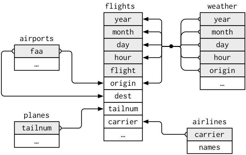
The values in the variable carrier in the flights data frame match the values in the variable carrier in the airlines data frame. In this case, we can use the variable carrier as a key variable to match the rows of the two data frames. Key variables are almost always identification variables that uniquely identify the observational units as we saw in Section 1.4.4. This ensures that rows in both data frames are appropriately matched during the join. Hadley and Garrett (Grolemund and Wickham 2017) created the diagram in Figure 3.7 to show how the different data frames in the nycflights23 package are linked by various key variables:
3.7.1 Matching key variable names
In both the flights and airlines data frames, the key variable we want to join/merge/match the rows by has the same name: carrier. Let’s use the inner_join() function to join the two data frames, where the rows will be matched by the variable carrier, and then compare the resulting data frames:
flights_joined <- flights |>
  inner_join(airlines, by = "carrier")
View(flights)
View(flights_joined)Observe that the flights and flights_joined data frames are identical except that flights_joined has an additional variable name. The values of name correspond to the airline companies’ names as indicated in the airlines data frame.
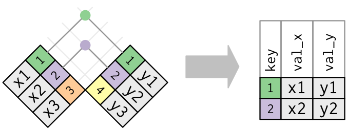
A visual representation of the inner_join() is shown in Figure 3.8. There are other types of joins available (such as left_join(), right_join(), outer_join(), and anti_join()), but the inner_join() will solve nearly all of the problems you’ll encounter in this book.
3.7.2 Different key variable names
Say instead you are interested in the destinations of all domestic flights departing NYC in 2023, and you ask yourself questions like: “What cities are these airports in?”, or “Is "ORD" Orlando?”, or “Where is "FLL"?”.
The airports data frame contains the airport codes for each airport:
View(airports)However, if you look at both the airports and flights data frames, you’ll find that the airport codes are in variables that have different names. In airports, the airport code is in faa, whereas in flights the airport codes are in origin and dest. This fact is further highlighted in the visual representation of the relationships between these data frames in Figure 3.7.
In order to join these two data frames by airport code, our inner_join() operation will use the by = c("dest" = "faa") argument with modified code syntax allowing us to join two data frames where the key variable has a different name:
flights_with_airport_names <- flights |>
  inner_join(airports, by = c("dest" = "faa"))
View(flights_with_airport_names)
Let’s construct the chain of pipe operators |> that computes the number of flights from NYC to each destination, but also includes information about each destination airport:
# A tibble: 118 × 9
   dest  num_flights airport_name             lat    lon   alt    tz dst   tzone
   <chr>       <int> <chr>                  <dbl>  <dbl> <dbl> <dbl> <chr> <chr>
 1 BOS         19036 General Edward Lawren…  42.4  -71.0    20    -5 A     Amer…
 2 ORD         18200 Chicago O'Hare Intern…  42.0  -87.9   672    -6 A     Amer…
 3 MCO         17756 Orlando International…  28.4  -81.3    96    -5 A     Amer…
 4 ATL         17570 Hartsfield Jackson At…  33.6  -84.4  1026    -5 A     Amer…
 5 MIA         16076 Miami International A…  25.8  -80.3     8    -5 A     Amer…
 6 LAX         15968 Los Angeles Internati…  33.9 -118.    125    -8 A     Amer…
 7 FLL         14239 Fort Lauderdale Holly…  26.1  -80.2     9    -5 A     Amer…
 8 CLT         12866 Charlotte Douglas Int…  35.2  -80.9   748    -5 A     Amer…
 9 DFW         11675 Dallas Fort Worth Int…  32.9  -97.0   607    -6 A     Amer…
10 SFO         11651 San Francisco Interna…  37.6 -122.     13    -8 A     Amer…
# ℹ 108 more rows
In case you didn’t know, "ORD" is the airport code of Chicago O’Hare airport and "FLL" is the main airport in Fort Lauderdale, Florida, which can be seen in the airport_name variable.
3.7.3 Multiple key variables
Say instead we want to join two data frames by multiple key variables. For example, in Figure 3.7, we see that in order to join the flights and weather data frames, we need more than one key variable: year, month, day, hour, and origin. This is because the combination of these 5 variables act to uniquely identify each observational unit in the weather data frame: hourly weather recordings at each of the 3 NYC airports.
We achieve this by specifying a vector of key variables to join by using the c() function. Recall from Section 1.2.1 that c() is short for “combine” or “concatenate.”
flights_weather_joined <- flights |>
  inner_join(weather, by = c("year", "month", "day", "hour", "origin"))
View(flights_weather_joined)
Learning Check
(LC3.13) Looking at Figure 3.7, when joining flights and weather (or, in other words, matching the hourly weather values with each flight), why do we need to join by all of year, month, day, hour, and origin, and not just hour?
hour repeats every day and at all three origins. You need year, month, day, hour, origin to uniquely identify the correct hourly record at the correct airport. hour is simply a value between 0 and 23; to identify a specific hour, we need to know which year, month, day and at which airport.
(LC3.14) What surprises you about the top 10 destinations from NYC in 2023?
Answers vary. Example: heavy traffic to Florida hubs and ORD/ATL; west-coast volumes lower/higher than intuition. Also, the high number of flights to Boston; wouldn’t it be easier and quicker to take the train?
3.7.4 Normal forms
The data frames included in the nycflights23 package are in a form that minimizes redundancy of data. For example, the flights data frame only saves the carrier code of the airline company; it does not include the actual name of the airline. For example, you’ll see that the first row of flights has carrier equal to UA, but it does not include the airline name “United Air Lines Inc.”
The names of the airline companies are included in the name variable of the airlines data frame. In order to have the airline company name included in flights, we could join these two data frames as follows:
joined_flights <- flights |>
  inner_join(airlines, by = "carrier")
View(joined_flights)
We are capable of performing this join because each of the data frames has keys in common to relate one to another: the carrier variable in both the flights and airlines data frames. The key variable(s) that we base our joins on are often identification variables as we mentioned previously.
This is an important property of what’s known as normal forms of data. The process of decomposing data frames into less redundant tables without losing information is called normalization. More information is available on Wikipedia.
Both dplyr and SQL we mentioned in the introduction of this chapter use such normal forms. Given that they share such commonalities, once you learn either of these two tools, you can learn the other very easily.
Learning Check
(LC3.15) What are some advantages of data in normal forms? What are some disadvantages?
Pros: less redundancy, consistent updates, smaller storage, clean joins. Cons: Need more joins, queries can be harder/slower, less convenient for quick, denormalized reporting.
3.8 Other verbs
Here are some other useful data-wrangling verbs:
-
select()only a subset of variables/columns. -
relocate()variables/columns to a new position. -
rename()variables/columns to have new names. - Return only the
top_n()values of a variable.
3.8.1 select variables
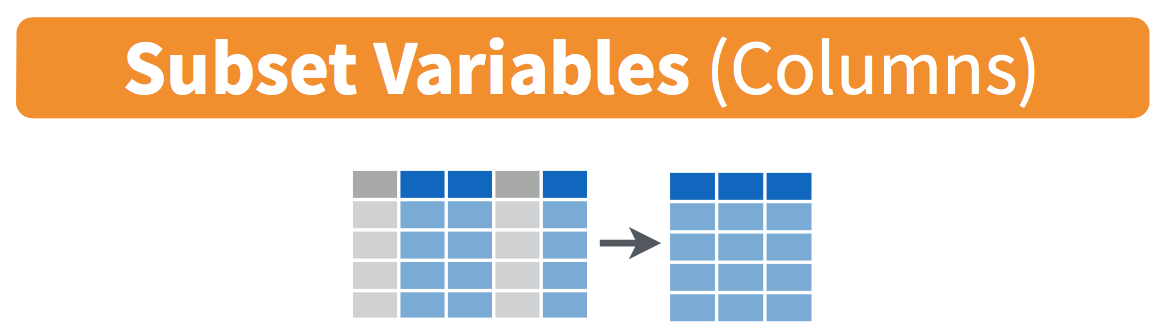
We’ve seen that the flights data frame in the nycflights23 package contains 19 different variables. You can identify the names of these 19 variables by running the glimpse() function from the dplyr package:
glimpse(flights)However, say you only need two of these 19 variables, say carrier and flight. You can select() these two variables:
flights |>
select(carrier, flight)This function makes it easier to explore large datasets since it allows us to limit the scope to only those variables we care most about. For example, if we select() only a smaller number of variables as is shown in Figure 3.9, it will make viewing the dataset in RStudio’s spreadsheet viewer more digestible.
Let’s say instead you want to drop, or de-select, certain variables. For example, consider the variable year in the flights data frame. This variable isn’t quite a “variable” because it is always 2023 and hence doesn’t change. Say you want to remove this variable from the data frame. We can deselect year by using the - sign:
flights_no_year <- flights |> select(-year)Another way of selecting columns/variables is by specifying a range of columns:
flight_arr_times <- flights |> select(month:day, arr_time:sched_arr_time)
flight_arr_times
This will select() all columns between month and day, as well as between arr_time and sched_arr_time, and drop the rest.
The helper functions starts_with(), ends_with(), and contains() can be used to select variables/columns that match those conditions. As examples,
Lastly, the select() function can also be used to reorder columns when used with the everything() helper function. For example, suppose we want the hour, minute, and time_hour variables to appear immediately after the year, month, and day variables, while not discarding the rest of the variables. In the following code, everything() will pick up all remaining variables:
flights_reorder <- flights |>
  select(year, month, day, hour, minute, time_hour, everything())
glimpse(flights_reorder)
3.8.2 relocate variables
Another (usually shorter) way to reorder variables is by using the relocate() function. This function allows you to move variables to a new position in the data frame. For example, if we want to move the hour, minute, and time_hour variables to appear immediately after the year, month, and day variables, we can use the following code:
3.8.3 rename variables
One more useful function is rename(), which as you may have guessed changes the name of variables. Suppose we want to only focus on dep_time and arr_time and change dep_time and arr_time to be departure_time and arrival_time instead in the flights_time_new data frame:
Note that in this case we used a single = sign within the rename(). For example, departure_time = dep_time renames the dep_time variable to have the new name departure_time. This is because we are not testing for equality like we would using ==. Instead we want to assign a new variable departure_time to have the same values as dep_time and then delete the variable dep_time. Note that new dplyr users often forget that the new variable name comes before the equal sign.
3.8.4 top_n values of a variable
We can also return the top n values of a variable using the top_n() function. For example, we can return a data frame of the top 10 destination airports using the example from Section 3.7.2. Observe that we set the number of values to return to n = 10 and wt = num_flights to indicate that we want the rows corresponding to the top 10 values of num_flights. See the help file for top_n() by running ?top_n for more information.
named_dests |> top_n(n = 10, wt = num_flights)Let’s further arrange() these results in descending order of num_flights:
Learning Check
(LC3.16) What are some ways to select all three of the dest, air_time, and distance variables from flights? Give the code showing how to do this in at least three different ways.
(LC3.17) How could one use starts_with(), ends_with(), and contains() to select columns from the flights data frame? Provide three different examples in total: one for starts_with(), one for ends_with(), and one for contains().
(LC3.18) Why might we want to use the select() function on a data frame?
To focus on relevant variables, declutter views, speed up downstream operations/joins, and reduce memory.
(LC3.19) Create a new data frame that shows the top 5 airports with the largest arrival delays from NYC in 2023.
top5_arr_delay <- flights |>
  group_by(dest) |>
  summarize(mean_arr_delay = mean(arr_delay, na.rm = TRUE), .groups="drop") |>
  arrange(desc(mean_arr_delay)) |>
  top_n(n = 5) |>
  # Useful for looking up the name of the airports!
  inner_join(airports, by = c("dest" = "faa")) |>
  # Can rename with select too!
  select(dest, airport_name = name, mean_arr_delay)
Selecting by mean_arr_delaytop5_arr_delay# A tibble: 5 × 3
dest airport_name mean_arr_delay
<chr> <chr> <dbl>
1 PSE Mercedita Airport 37.6
2 ANC Ted Stevens Anchorage International Airport 36.5
3 RNO Reno Tahoe International Airport 34.4
4 ABQ Albuquerque International Sunport 26.7
5 ONT Ontario International Airport 26.1Quick checks
Ten questions to assess your understanding. Several are designed around common misconceptions — read each option carefully before peeking at the answer.
Q3-1. Which dplyr verb keeps only the rows where carrier == "DL"?
Q3-2. What does this pipeline return?
- A data frame with one row per origin
- A vector of departure delays
- The original
flightsdata frame - An error, because
dep_delayhas missing values
(a) group_by() + summarize() collapses the data to one row per group.
Q3-3. Why do many summarize() calls include na.rm = TRUE?
- To increase the precision of the result
- To remove negative values
- To exclude missing values
- To round to whole numbers
(c) na.rm = TRUE tells the summary function to skip NA values. Without it, any missing value will cause the entire summary to return NA. (But always think about why the values are missing before reaching for it.)
Q3-4. What’s the difference between filter(flights, carrier == "DL") and filter(flights, carrier = "DL")?
- The second triggers an error
- They’re equivalent
- The first returns Delta flights; the second returns all flights
- Both work but the second is slower
(a) == compares; = assigns argument values. Mixing them up is one of the most common dplyr errors.
Q3-5. After running flights |> mutate(gain = dep_delay - arr_delay) without <-, the flights data frame:
- Is unchanged
- Has the new
gaincolumn added - Has the new column AND its previous columns are removed
- Errors
(a) Verbs like mutate() return a modified copy. To keep it, you must reassign with <-: flights <- flights |> mutate(...). Without that, the modified version is printed and discarded.
Q3-6. flights |> arrange(dep_delay) returns rows sorted by departure delay. The first row is most likely:
- The flight with the largest positive
dep_delay - A randomly chosen flight
- A flight with
dep_delayof exactly 0 - The flight with the most negative
dep_delay
(d) arrange() sorts ascending by default. The smallest value (most negative) comes first, meaning the flight that left earliest relative to its scheduled departure time. Use arrange(desc(dep_delay)) for largest first.
Q3-7. flights |> inner_join(airlines, by = "carrier") returns:
- The union of both data frames
- Only rows from
flightswhosecarriervalue also appears inairlines - All rows from
airlines, with flight info added - All rows from
flights, with airline info filled in where matched (NAotherwise)
(b) Inner join keeps only rows matched in BOTH tables. (d) describes a left_join; (c) is a right_join. With nycflights23, every carrier in flights is in airlines, so the visible row count is the same, but the conceptual difference matters when keys don’t all match.
Q3-8. flights |> filter(dep_delay > 60 | arr_delay > 60) returns rows where:
- An error, because
|is not a valid operator - BOTH
dep_delayandarr_delayexceed 60 - Neither delay exceeds 60
- EITHER
dep_delayorarr_delayexceeds 60
(d) | is the OR operator in R. & is AND. Confusing the two is a common student error.
Q3-9. After flights |> group_by(origin), what visible change happens to the data frame?
- A new column appears
- Rows with
NAare dropped - Nothing visible changes
- Rows are reordered by origin
(c) group_by() is a labeling step. The data frame looks the same; downstream verbs see the grouping and act per-group.
Q3-10. Compare these two expressions:
flights |> filter(carrier == "DL") |> summarize(mean_delay = mean(dep_delay, na.rm = TRUE))
summarize(filter(flights, carrier == "DL"), mean_delay = mean(dep_delay, na.rm = TRUE))
Which statement is correct?
- They give different answers because piping changes what each function “sees”
- errors because
|>can’t be used with multiple verbs
- errors because
- They produce exactly the same result
- errors because
summarize()needs the grouped data first
- errors because
(c) The pipe |> takes the value on its left and passes it as the first argument of the function on its right, so a chain of |>s is just shorthand for the same nested call. Prefer the piped form when you have three or more verbs in a row; it reads top-to-bottom like a recipe instead of inside-out.
dplyr verb |
What it does | Quick example |
|---|---|---|
filter() |
Keep rows matching a condition | flights |> filter(carrier == "DL") |
select() |
Pick / drop / reorder columns | flights |> select(carrier, flight) |
mutate() |
Add or transform a column | flights |> mutate(gain = dep_delay - arr_delay) |
arrange() (use desc() for descending) |
Sort rows | flights |> arrange(desc(dep_delay)) |
summarize() |
Collapse to summary statistics | flights |> summarize(mean = mean(dep_delay, na.rm = TRUE)) |
group_by() |
Group rows so a verb operates per-group | flights |> group_by(carrier) |> summarize(...) |
inner_join(y, by = "k") |
Combine two tables on shared key column | flights |> inner_join(airlines, by = "carrier") |
|> |
Pipe: pass the result of the LHS to the RHS as its first argument | flights |> filter(...) |> summarize(...) |
Exercises
The end-of-chapter exercises mix two datasets:
-
olympic_athletesandmedal_tablefrom theolympicAthletespackage (introduced in Chapter 2). -
episodesfrom thestevespackage — a tidied snapshot of every episode of Rick Steves’ Europe (159 rows × 38 columns) covering 2000–2025. Variables includeseason,primary_country,region,imdb_rating,imdb_votes,original_air_date, andtheme_tags. Install it once with:
install.packages("steves")Difficulty stars: ★ warm-up, ★★ standard application, ★★★ critical thinking. Solutions are available to instructors separately.
Data source (episodes, from the steves package). Source: Rick Steves’ Europe (compiled dataset). Note: This dataset was created from public sources for teaching purposes and is not an official or verified Rick Steves’ Europe dataset.
Setup
EX3.1 (★) Meet the data. Load steves and get to know this chapter’s dataset two ways. First run ?episodes (the same page lives on the package website at https://moderndive.github.io/steves/reference/episodes.html):
- What is the observational unit, and what span of the show does the data cover?
- Where do the values come from, and what does the documentation caution about how “official” this dataset is?
Then run glimpse(episodes):
- How many rows and columns? Name three numerical and three categorical variables.
EX3.2 (★) Predict, then verify with min() and max(): what are the smallest and largest values of imdb_rating in episodes? And of season?
EX3.3 (★) original_air_date has type Date, not character. Why does storing it as a true date matter when you arrange() episodes into chronological order, compared with storing the same values as text?
The pipe operator |>
EX3.4 (★) Take this nested expression and rewrite it as a |>-piped chain. Verify the two produce identical output.
In one sentence, why does the piped version usually read more naturally for humans than the nested one?
filter()
EX3.5 (★) Filter olympic_athletes to athletes from sport == "Swimming" who won a Gold medal. How many rows result?
EX3.6 (★) Filter episodes to those where primary_country == "Italy". How many Italy episodes does the show have?
EX3.7 (★) Filter episodes to highly-rated AND well-watched episodes: imdb_rating >= 8 AND imdb_votes >= 25.
EX3.8 (★) Filter episodes to the union: episodes about "Italy" OR "France". Use %in%.
EX3.9 (★★) Filter olympic_athletes to the 2024 Summer Games (year == 2024 & season == "Summer"). How many athlete-event participations (rows) remain? Use n() inside summarize() (each row is one athlete in one event).
group_by() + summarize()
EX3.10 (★★) Compute the mean height per sport (drop NAs with na.rm = TRUE). Show the 10 sports with the tallest mean.
EX3.11 (★★) Using medal_table for the 2018-2026 Games (year >= 2018), compute the total medals per NOC (National Olympic Committee). Group by both noc and country so the readable country name shows alongside the three-letter code, then show the top 10 with top_n().
EX3.12 (★★) From episodes, compute the median imdb_rating per region. Which region rates highest?
EX3.13 (★★) Count the number of episodes per season of Rick Steves’ Europe. Plot it as a barplot.
EX3.14 (★★) From olympic_athletes, count the number of athlete-event participations (rows) per noc with n(), then show the 10 nocs with the most.
EX3.15 (★★★) Compute mean age per sport, but only for sports with at least 1,000 athlete-rows. Why is the second filter important?
EX3.16 (★★) For each Games (year × season), count the number of athlete-event participations (rows) with n(). Has the number of participations grown over time? Plot it.
mutate()
EX3.17 (★★) Add a height_in column to olympic_athletes: convert height (cm) to inches (1 inch ≈ 2.54 cm).
EX3.18 (★★) Add a bmi column to olympic_athletes computed from weight (kg) and height (cm) as weight / (height / 100)^2. Show the first few rows where bmi is non-missing.
EX3.19 (★★) Add a logical column won_medal to olympic_athletes that is TRUE for any non-missing medal. What proportion of athlete-rows won a medal?
EX3.20 (★★) For the 2018-2026 Games (year >= 2018), add a gold_share column to medal_table computed as gold / (gold + silver + bronze). Display the resulting data frame so the new column is visible.
arrange()
EX3.21 (★★) Show the 10 oldest athletes (by age, descending) among Games from 2000 onward: first filter(year >= 2000) (which also drops the long-defunct Art Competitions, so you get the oldest real competitors rather than elderly artists), then arrange(desc(age)).
EX3.22 (★★) Show the 5 highest-rated episodes of Rick Steves’ Europe. Print only season, episode_in_season, title, imdb_rating.
EX3.23 (★★) Sort episodes first by season ascending, then imdb_rating descending, and inspect rows 1–10. Those ten rows are the strongest episodes of the earliest season, do their ratings vary a lot, or is season 1 uniformly strong? Then re-sort by imdb_rating alone (descending): which season(s) do the very highest-rated episodes of the whole series come from, and what might that suggest about when the show hit its stride?
EX3.24 (★★★) Medal efficiency (a group_by() → summarize() → mutate() → arrange() pipeline). The USA and China win the most total medals, but which countries are most efficient, converting the fewest participations into the most medals? For the 2024 Summer Games, mutate() a logical won_medal = !is.na(medal) flag (as in EX 3.19), then group_by(noc) and summarize() each country’s number of athlete-event participations (n()) and number of medal-winning rows (sum(won_medal)), then mutate() a medal_per_participation percentage and arrange() by it. Re-run keeping only countries with at least 50 participations, so a single medal-winning row can’t read as 100%. Which country tops the efficiency ranking, and how does it compare with the USA and China? (These are athlete-event row counts; for exact distinct-athlete counts, see Extension EX 3.71.)
join()
EX3.25 (★★★) editions carries per-Games metadata for every Olympics. First keep just the five 2018-2026 Games with editions_since_2018 <- editions |> filter(year >= 2018), then use inner_join() to attach editions_since_2018 to olympic_athletes. What is the resulting row count, and why is it so much smaller than the number of rows in olympic_athletes?
EX3.26 (★) editions carries one row per Olympic Games, including participants (how many athletes competed at that Games overall). Attach that count to every curler in curling_athletes. First narrow the lookup with games_size <- editions |> select(games, participants), then inner_join() it onto curling_athletes by games. How many rows come back, and why is that the number you should expect?
EX3.27 (★★) A colleague sends you a slimmed-down lookup table where the Games column has been renamed: games_lookup <- editions |> select(games_code = games, host_city = city_english). Attach host_city to curling_athletes. The key means the same thing on both sides but is spelled differently, so by = "games" will error. Fix it, and say which of the two names survives in the result.
EX3.28 (★★) Join the whole of editions onto curling_athletes with by = "games" and look at the column names. Four of them come back as .x/.y pairs. Explain what happened, then fix it so no suffixed columns appear, without dropping any columns first. Does your fix change the number of rows?
Other verbs (select(), relocate(), rename())
EX3.29 (★) From olympic_athletes, select only the identifier columns (id, name) plus the medal-related columns (medal, event, sport, year).
EX3.30 (★) Use a tidyselect helper (starts_with, contains, ends_with) to keep only the IMDB-related columns of episodes.
EX3.31 (★) Drop the image_url and tvmaze_url columns from episodes using select(-...).
EX3.32 (★★) Build a small wrangling pipeline on medal_table that uses three of the Other verbs from Section 3.8, select(), relocate(), and rename(). Goal: keep only the columns noc, country, gold, silver, bronze, total; rename noc to iso_code; reorder columns so country comes first. Show the first 5 rows of the result.
Critical thinking and open exploration
EX3.33 (★★) Run mean(olympic_athletes$height) (without na.rm). What do you get, and why?
EX3.34 (★★★) Compare two coding styles for the same task: (a) save each intermediate result to a variable, (b) chain everything with |>. Pick a 3-step dplyr chain and write it both ways. Which is easier to modify? Which is easier to debug?
EX3.35 (★★★) Pick two countries (e.g., "USA" and "GBR") and produce a single linegraph of their total medals across the 2018–2026 Games. What story does the chart tell?
EX3.36 (★★★) From episodes, compute episodes per primary_country and identify the most-featured country. Then compute the same with geo_match == "full" (only fully geo-resolved episodes), does the leader change?
EX3.37 (★★★) At the Tokyo 2020 Summer Games, which sports fielded the most athletes? Filter olympic_athletes to 2020 Summer, count athlete-event rows per sport, and show the top 8. What about the ranking surprises you?
EX3.38 (★★★) EX 3.37’s Tokyo top-8 included Hockey, surprising if you were picturing ice rinks at a Summer Games. Investigate with taught tools: filter() olympic_athletes to the sports "Hockey" and "Ice Hockey", then group_by(sport, season) and summarize(n = n()).
- What does the sport called
"Hockey"mean in Olympic data?
- What does the sport called
- Your table will also show
"Ice Hockey"rows in a Summer season. Is that a data error? Before deciding, check whichyearthose rows come from and compare against the first Winter Games ineditions.
- Your table will also show
EX3.39 (★★★) Open exploration: combining at least two dplyr verbs and one of the two datasets, find one finding that surprises you. State your finding in one sentence above the supporting code.
Visualizations unlocked by dplyr wrangling
EX3.40 (★★) height and weight in olympic_athletes have many NA values, especially for older Games. Predict, without running code, why this is. Then use summarize() and mean(is.na(...)) to compute the proportion of NAs in each of those two columns.
EX3.41 (★★★) EX 3.40 computed one overall NA rate for height, but missingness isn’t spread evenly across Olympic history. Group the athletes into 20-year “generations” with mutate(generation = floor(year / 20) * 20). Here floor(...) is base R’s round-down function; the book doesn’t cover it, so the starter comment walks through an example (1936 → 1920, 2024 → 2020). Then group_by(generation) and summarize() the proportion of missing height per generation, and draw a linegraph of that proportion over the generations. Describe the shape: which eras are worst, and why does the most recent generation break the improving trend?
EX3.42 (★★) Using medal_table, plot the total medals (gold + silver + bronze) won by "CAN" (Canada) across the five 2018-2026 Games as a linegraph (year on the x-axis). You’ll need filter() → mutate() → ggplot(). Then read your graph: does anything interesting stand out when you trace Canada’s line across the five Games? (Keep in mind which years are Winter Games and which are Summer.)
EX3.43 (★★) Compute the number of athlete-event participations (rows) per Games in olympic_athletes with n() and plot it as a linegraph against year. Filter to a single season (Summer or Winter), combining them would mix two cycles.
EX3.44 (★★) For one sport of your choice, plot mean height per year over time. Has the typical height of athletes in that sport grown, shrunk, or stayed flat?
EX3.45 (★★) Filter to the top-5 NOCs in medal_table (by total medals across all Games), then use facet_wrap(~ noc) to show a geom_col barplot of medal totals per Games for each NOC, filled by season. Look closely at how the bars change over time: for earlier years each bar splits into two stacked segments, but for later years there’s just one. What change in the Olympic schedule explains this?
EX3.46 (★★) Identify the 5 sports with the most athletes by group_by(sport), summarize(n_athletes = n()), then top_n(n = 5, wt = n_athletes). Build boxplots of height for just those five sports. Which sport has the highest median height? Which has the largest IQR?
EX3.47 (★★) Use medal_table to find the 10 NOCs with the most total medals across all five 2018-2026 Games combined. Display them as a horizontal bar chart, sorted descending.
EX3.48 (★★) Build a barplot of medal counts for the 2024 Summer Games only (one bar per top-10 NOC, using top_n()). What’s the top NOC?
EX3.49 (★★) Using medal_table and the top-5 NOCs by total medals, build a dodged (side-by-side) barplot of medal counts split by season, two bars per NOC (Summer and Winter), color-filled by season.
Need a hint?
Summarize by noc and season, then geom_col(position = "dodge").
EX3.50 (★★★) Build a chart that visualizes the rise of female participation in the Summer Olympics over time. State your finding in one sentence above the chart.
Need a hint?
Count athlete-event participations (rows) per year × sex with n(), filter to Summer.
EX3.51 (★★★) Explore how athletes’ average height has changed over time across several sports. Try a few from this menu: volleyball, gymnastics, rowing, swimming, fencing, shooting. Some show a dramatic change, some barely move. Pick the one with the most dramatic change and build a chart that supports it. Acknowledge any caveats, e.g., missing height data for older Games (use the post-summary filter() to drop years with too few observations to trust).
EX3.52 (★★★) Reuniting the 1956 Summer Games. Back in Chapter 2 (EX 2.13-2.14) the Summer participation linegraph plunged at 1956, because the 1956 Summer Games appear as two rows in editions (the main Melbourne Games plus a separate Stockholm edition that hosted only the equestrian events), and the line dips through the tiny 158-athlete Stockholm point. Use group_by(year, season) and summarize() to combine the two 1956 rows into one Games (sum the participants), then compare the combined 1956 total with the Summer Games of 1948, 1952, and 1960. Does combining the split rows fully explain the dip, or was 1956 a genuinely smaller Games?
Extensions
The exercises below deliberately introduce functions and concepts beyond what this chapter teaches — log transformations, predict(), new packages, foreshadowing later chapters. They are optional, aimed at readers who want to push further. The main Exercises and Quick checks above stick strictly to what this chapter covers.
EX3.53 (◆◆◆) Turning the wide gold/silver/bronze columns into a medal_type column requires pivot_longer() from Ch 4.
Modify your top-10 plot (from EX 3.47) to stack gold/silver/bronze in each bar.
Need a hint?
pivot_longer() first, then map fill = medal_type.
EX3.54 (◆◆) Why this is an Extension: the gold/silver/bronze counts live in three separate columns of medal_table, but ggplot() wants them stacked in one column with a label alongside, and reshaping columns into that longer form takes pivot_longer(), a Chapter 4 tool previewed here.
Take the stacked gold/silver/bronze barplot from EX 3.53 and rebuild it with position = "fill" so each NOC’s bar reaches 100 %. Compare the two charts: what new question does the proportional version answer (that the stacked-counts version cannot), and conversely what does the original show that gets hidden when you switch to proportions?
EX3.55 (◆◆◆) Counting NAs across columns needs summarize(across()) + pivot_longer() to reshape into a plottable frame.
Chapter 2 didn’t show NA visualization. Build a barplot showing the count of NAs per column in olympic_athletes. Which columns have the most missingness? Why might that be?
EX3.56 (◆◆) case_when() for multi-level conditional mutates. When you want to derive a new categorical column from a numeric one with more than two buckets, case_when() is cleaner than nesting ifelse()s. Build an age_group column on olympic_athletes with buckets "under 20", "20s", "30s", "40+", then count athletes in each.
EX3.57 (◆◆) if_else() for boolean conditional mutates. When the condition has exactly two outcomes, if_else(condition, value_if_TRUE, value_if_FALSE) is the cleanest tool. It’s strict about both branches having the same type, which catches subtle bugs that base R’s ifelse() silently lets through. Try building an is_medalist column on olympic_athletes ("yes" if medal is not NA, "no" otherwise), then count how many athlete-rows are in each.
EX3.58 (◆◆) The slice_*() family. Section 3.8.4 introduced top_n(); the dplyr ecosystem now favors a family of slice_*() verbs that read more clearly and have explicit variants. slice_max(col, n)/slice_min(col, n) for top/bottom by a column, slice_head(n)/slice_tail(n) for first/last rows, slice_sample(n) for a random subset. Try each above. For “top 10 NOCs by medals at Paris 2024,” which would you reach for first?
EX3.59 (◆◆) count() as a summarize(n = n()) shortcut. The pattern group_by(col) |> summarize(n = n()) |> arrange(desc(n)) is so common dplyr provides count(col, sort = TRUE) as a one-liner. Use it on olympic_athletes to find the 5 most-represented sports. When you need more than one summary stat per group (e.g., mean and SD), stick with group_by() + summarize(); for pure row counts, count() wins.
EX3.60 (◆◆◆) across() for applying a function to many columns. Writing summarize(mean_age = mean(age, na.rm = TRUE), mean_height = ..., mean_weight = ...) for many columns is tedious. across(<cols>, <fn>) applies the same function to multiple columns at once. The starter snippet computes mean and SD for age, height, weight all in one summarize. (We mentioned this in passing in EX 3.53, here’s the dedicated walk-through.)
EX3.61 (◆◆) bind_rows() and bind_cols(). When you have two data frames with the same columns and want to stack them vertically, use bind_rows(). For two frames with the same rows in the same order that you want to glue side-by-side, use bind_cols() (rare, usually a join is safer). Try bind_rows() to combine 2024 Summer and 2022 Winter medal tables. Why is bind_rows() safer than rbind() (the base-R equivalent)?
EX3.62 (◆◆◆) String manipulation with stringr. Real-world data is full of text that needs cleaning. The stringr package provides a consistent family of str_*() functions: str_detect() (does the string match this pattern?), str_replace() (swap one pattern for another), str_to_lower(), str_trim(). Use the starter snippet to flag team events in olympic_athletes$event. Briefly: when would you want regular expressions in the pattern argument vs. literal strings?
EX3.63 (◆◆◆) Date handling with lubridate. Dates look like strings but behave like numbers, and parsing them by hand with substr() and as.numeric() is error-prone. The lubridate package gives you tidy parsers (ymd(), mdy(), dmy()) and extractors (year(), month(), wday()). Use it on episodes$original_air_date to add year, month, and weekday columns. Which weekday did Rick Steves’ Europe air on most often?
EX3.64 (◆◆◆) Splitting columns with separate_wider_delim(). When one column packs two pieces of info (e.g., "2024 Summer"), tidyr::separate_wider_delim() splits it on a delimiter into named output columns. Apply it to medal_table$games. (Compare your result to medal_table’s existing year and season columns, same info, but you’ve reconstructed it from the combined string.)
EX3.65 (◆◆◆) rowwise() for row-by-row computation. Most dplyr verbs are vectorized (operate on whole columns at once), which is fast but awkward when you need a per-row reduction across multiple columns. rowwise() switches dplyr to per-row mode. The starter snippet finds, for each (Games × NOC) row, which medal color the country won the most of. Always pair rowwise() with ungroup() when you’re done, otherwise subsequent verbs stay slow.
EX3.66 (◆◆) fct_reorder() as the tidyverse swap for reorder(). Earlier exercises (e.g., EX 3.48) used base R’s reorder(noc, total) inside aes(...) to sort a categorical axis by a numeric column. The tidyverse package forcats provides fct_reorder(), the same idea, but it lives in the same family as fct_relevel(), fct_recode(), and other fct_*() helpers, so it composes cleanly with other factor verbs you’ll reach for in larger pipelines. Build a horizontal bar chart of the 10 NOCs with the most medals at the 2024 Summer Games two ways, once sorting the bars with reorder(noc, total) and once with fct_reorder(noc, total), and compare them. Are the plots identical? When does it matter which one you use?
EX3.67 (◆◆) lubridate::year() for date-component extraction. When you have a Date column and need just the year (or month, day, weekday), the lubridate package exposes one verb per component, year(), month(), day(), wday(). These compose cleanly inside mutate() chains. episodes already has a precomputed air_year column, which makes this a perfect cross-check: derive year_recomputed = year(original_air_date) yourself and confirm the two columns match.
EX3.68 (◆◆◆) left_join() (an Extension). Chapter 3 teaches only inner_join(); left_join(), which keeps every row of the left data frame, filling unmatched columns with NA, is only name-dropped in Section 3.7. Use left_join() with editions_since_2018 (editions |> filter(year >= 2018)) instead. What’s the row count, and why is it different from the inner-join result?
EX3.69 (◆◆◆) anti_join() (a filtering join, an Extension). Chapter 3 teaches only inner_join(); anti_join(), which keeps the rows of x without a match in y, adding none of y’s columns, is only name-dropped in Section 3.7. Use anti_join() between olympic_athletes and medal_table (joining on year/year and noc/noc) to find athletes whose NOC did not appear in medal_table for that Games. What does this tell you about coverage?
EX3.70 (◆◆◆) semi_join() (a filtering join, an Extension). Chapter 3 teaches only inner_join(), and semi_join() appears nowhere in the book: it keeps the rows of x that have a match in y, without adding any of y’s columns. Use semi_join() to keep only the athletes from countries that appear in medal_table (i.e., NOCs that won at least one medal at that Games). How many rows remain?
EX3.71 (◆◆) n_distinct() for exact distinct counts. Several earlier exercises counted athlete-rows with n() (one row per athlete-event participation). To count distinct values instead, the number of different athletes, events, or countries, use n_distinct(col) inside summarize(). For each noc, compute both the number of distinct athletes (n_distinct(id)) and the number of rows (n()) in one summary. When, and why, do the two answers differ (cf. EX3.14, which counts rows)?
EX3.72 (◆◆◆) Olympic art?! From 1912 to 1948 the Olympics awarded real medals for art inspired by sport, architecture, literature, music, painting, and sculpture. Those entries are still in olympic_athletes under sport == "Art Competitions".
-
filter()to the art competitions, thensummarize()how many rows there are and the range ofyears they span.
-
- Add a
mutate()flagis_art = sport == "Art Competitions", thengroup_by()it andsummarize()the median age of art competitors versus everyone else, how do they compare?
- Add a
-
arrange()the art competitors byage(descending) to find the oldest, how old were they, and in which event?
-
Finally, a histogram of every Olympian’s age has a surprising little bump of competitors in their 70s, 80s, and 90s. What does your answer explain about that bump, and why might you filter(sport != "Art Competitions") before studying athletic ages?
EX3.73 (◆◆) Density of a derived variable (mutate() + geom_density()). A density plot (the smoothed alternative to a histogram, geom_density() in place of geom_histogram()) only looks smooth for a continuous variable; the raw integer columns (height, weight, age) are too granular and give a jagged, spiky curve. Use mutate() to add a body-mass index column bmi = weight / (height/100)^2 (a ratio, so it takes continuous decimal values), drop the missing values with filter(), and draw its density. Roughly where does BMI peak for Olympic athletes, and why is the derived bmi a smoother candidate for a density plot than the integer weight on its own?
3.9 Conclusion
3.9.1 Summary table
Let’s recap our data-wrangling verbs in Table 3.2. Using these verbs and the pipe |> operator from Section 3.1, you’ll be able to write easily legible code to perform almost all the data wrangling and data transformation necessary for the rest of this book.
| Verb | Data wrangling operation |
|---|---|
filter() |
Pick out a subset of rows |
summarize() |
Summarize many values to one using a summary statistic function like mean(), median(), etc. |
group_by() |
Add grouping structure to rows in data frame. Note this does not change values in data frame, rather only the meta-data |
mutate() |
Create new variables by mutating existing ones |
arrange() |
Arrange rows of a data variable in ascending (default) or descending order |
inner_join() |
Join/merge two data frames, matching rows by a key variable |
Learning Check
(LC3.20) Let’s now put your newly acquired data-wrangling skills to the test!
An airline industry measure of a passenger airline’s capacity is the available seat miles, which is equal to the number of seats available multiplied by the number of miles or kilometers flown summed over all flights.
For example, let’s consider the scenario in Figure 3.10. Since the airplane has 4 seats and it travels 200 miles, the available seat miles are \(4 \times 200 = 800\).
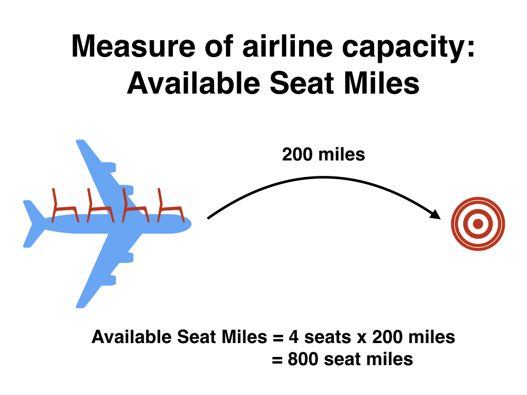
Extending this idea, let’s say an airline had 2 flights using a plane with 10 seats that flew 500 miles and 3 flights using a plane with 20 seats that flew 1000 miles, the available seat miles would be \(2 \times 10 \times 500 + 3 \times 20 \times 1000 = 70,000\) seat miles.
Using the datasets included in the nycflights23 package, compute the available seat miles for each airline sorted in descending order. After completing all the necessary data-wrangling steps, the resulting data frame should have 14 rows (one for each airline) and 2 columns (airline name and available seat miles). Here are some hints:
-
Crucial: Unless you are very confident in what you are doing, it is worthwhile not starting to code right away. Rather, first sketch out on paper all the necessary data wrangling steps not using exact code, but rather high-level pseudocode that is informal yet detailed enough to articulate what you are doing. This way you won’t confuse what you are trying to do (the algorithm) with how you are going to do it (writing
dplyrcode). - Take a close look at all the datasets using the
View()function:flights,weather,planes,airports, andairlinesto identify which variables are necessary to compute available seat miles. - Figure 3.7 showing how the various datasets can be joined will also be useful.
- Consider the data-wrangling verbs in Table 3.2 as your toolbox!
-
Crucial: Unless you are very confident in what you are doing, it is worthwhile to not starting coding right away, but rather first sketch out on paper all the necessary data wrangling steps not using exact code, but rather high-level pseudocode that is informal yet detailed enough to articulate what you are doing. This way you won’t confuse what you are trying to do (the algorithm) with how you are going to do it (writing
dplyrcode). - Take a close look at all the datasets using the
View()function:flights,weather,planes,airports, andairlinesto identify which variables are necessary to compute available seat miles. - Figure 3.7 above showing how the various datasets can be joined will also be useful.
- Consider the data wrangling verbs in Table 3.2 as your toolbox!
Solution: Here are some examples of student-written pseudocode. Based on our own pseudocode, let’s first display the entire solution.
# A tibble: 13 × 2
carrier ASM
<chr> <dbl>
1 UA 18753552904
2 B6 18302094316
3 DL 15282765973
4 AA 11173950579
5 NK 3880566315
6 YX 3512338372
7 AS 2974953367
8 9E 2501279760
9 WN 1986242879
10 HA 683807124
11 OO 325167024
12 F9 230428926
13 MQ 16311790Let’s now break this down step-by-step. To compute the available seat miles for a given flight, we need the distance variable from the flights data frame and the seats variable from the planes data frame, necessitating a join by the key variable tailnum as illustrated in Figure 3.7. To keep the resulting data frame easy to view, we’ll select() only these two variables and carrier:
flights |>
inner_join(planes, by = "tailnum") |>
select(carrier, seats, distance)# A tibble: 424,068 × 3
carrier seats distance
<chr> <int> <dbl>
1 UA 149 2500
2 DL 222 760
3 B6 200 1576
4 B6 20 636
5 UA 149 488
6 AA 162 1085
7 B6 246 1576
8 AA 162 719
9 UA 178 1400
10 NK 190 1065
# ℹ 424,058 more rowsNow for each flight we can compute the available seat miles ASM by multiplying the number of seats by the distance via a mutate():
flights |>
inner_join(planes, by = "tailnum") |>
select(carrier, seats, distance) |>
# Added:
mutate(ASM = seats * distance)# A tibble: 424,068 × 4
carrier seats distance ASM
<chr> <int> <dbl> <dbl>
1 UA 149 2500 372500
2 DL 222 760 168720
3 B6 200 1576 315200
4 B6 20 636 12720
5 UA 149 488 72712
6 AA 162 1085 175770
7 B6 246 1576 387696
8 AA 162 719 116478
9 UA 178 1400 249200
10 NK 190 1065 202350
# ℹ 424,058 more rowsNext we want to sum the ASM for each carrier. We achieve this by first grouping by carrier and then summarizing using the sum() function:
# A tibble: 13 × 2
carrier ASM
<chr> <dbl>
1 9E 2501279760
2 AA 11173950579
3 AS 2974953367
4 B6 18302094316
5 DL 15282765973
6 F9 230428926
7 HA 683807124
8 MQ 16311790
9 NK 3880566315
10 OO 325167024
11 UA 18753552904
12 WN 1986242879
13 YX 3512338372However, because for certain carriers certain flights have missing NA values, the resulting table also returns NA’s. We can eliminate these by adding a na.rm = TRUE argument to sum(), telling R that we want to remove the NA’s in the sum. We saw this in Section 3.3:
# A tibble: 13 × 2
carrier ASM
<chr> <dbl>
1 9E 2501279760
2 AA 11173950579
3 AS 2974953367
4 B6 18302094316
5 DL 15282765973
6 F9 230428926
7 HA 683807124
8 MQ 16311790
9 NK 3880566315
10 OO 325167024
11 UA 18753552904
12 WN 1986242879
13 YX 3512338372Finally, we arrange() the data in desc()ending order of ASM.
# A tibble: 13 × 2
carrier ASM
<chr> <dbl>
1 UA 18753552904
2 B6 18302094316
3 DL 15282765973
4 AA 11173950579
5 NK 3880566315
6 YX 3512338372
7 AS 2974953367
8 9E 2501279760
9 WN 1986242879
10 HA 683807124
11 OO 325167024
12 F9 230428926
13 MQ 16311790While the above data frame is correct, the IATA carrier code is not always useful. For example, what carrier is WN? We can address this by joining with the airlines dataset using carrier is the key variable. While this step is not absolutely required, it goes a long way to making the table easier to make sense of. It is important to be empathetic with the ultimate consumers of your presented data!
flights |>
  inner_join(planes, by = "tailnum") |>
  select(carrier, seats, distance) |>
  mutate(ASM = seats * distance) |>
  group_by(carrier) |>
  summarize(ASM = sum(ASM, na.rm = TRUE)) |>
arrange(desc(ASM)) |>
# Added:
inner_join(airlines, by = "carrier") |>
select(-carrier)# A tibble: 13 × 2
ASM name
<dbl> <chr>
1 18753552904 United Air Lines Inc.
2 18302094316 JetBlue Airways
3 15282765973 Delta Air Lines Inc.
4 11173950579 American Airlines Inc.
5 3880566315 Spirit Air Lines
6 3512338372 Republic Airline
7 2974953367 Alaska Airlines Inc.
8 2501279760 Endeavor Air Inc.
9 1986242879 Southwest Airlines Co.
10 683807124 Hawaiian Airlines Inc.
11 325167024 SkyWest Airlines Inc.
12 230428926 Frontier Airlines Inc.
13 16311790 Envoy Air 3.9.2 Additional resources
An R script file of all R code used in this chapter is available here.
In the online Appendix C, we provide a page of data wrangling ‘tips and tricks’ consisting of the most common data wrangling questions we’ve encountered in student projects (shout out to Dr. Jenny Smetzer for her work setting this up!):
- Dealing with missing values
- Reordering bars in a barplot
- Showing money on an axis
- Changing values inside cells
- Converting a numerical variable to a categorical one
- Computing proportions
- Dealing with %, commas, and dollar signs
However, to provide a tips and tricks page covering all possible data wrangling questions would be too long to be useful!
If you want to further unlock the power of the dplyr package for data wrangling, we suggest that you check out RStudio’s “Data Transformation with dplyr” cheatsheet. This cheatsheet summarizes much more than what we’ve discussed in this chapter, in particular more intermediate level and advanced data-wrangling functions, while providing quick and easy-to-read visual descriptions. In fact, many of the diagrams illustrating data wrangling operations in this chapter, such as Figure 3.1 on filter(), originate from this cheatsheet.
In the current version of RStudio in 2025, you can access this cheatsheet by going to the RStudio Menu Bar -> Help -> Cheatsheets -> “Data Transformation with dplyr.” You can see a preview in the figure below.
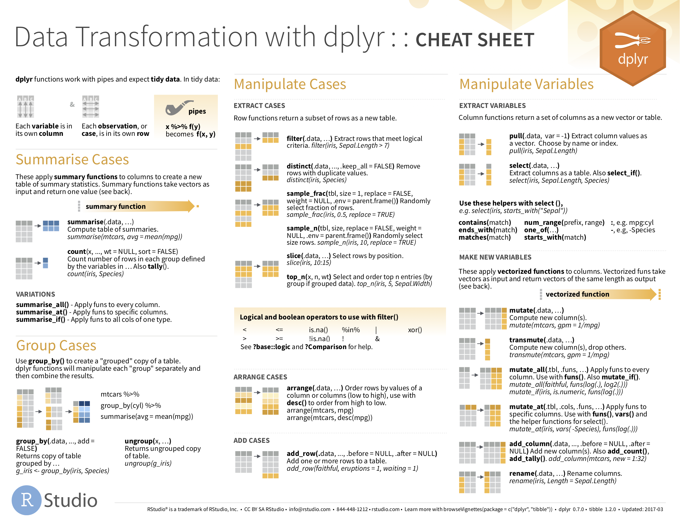
On top of the data-wrangling verbs and examples we presented in this section, if you’d like to see more examples of using the dplyr package for data wrangling, check out Chapter 5 of R for Data Science (Grolemund and Wickham 2017).
3.9.3 What’s to come?
So far in this book, we’ve explored, visualized, and wrangled data saved in data frames. These data frames were saved in a spreadsheet-like format: in a rectangular shape with a certain number of rows corresponding to observations and a certain number of columns corresponding to variables describing these observations.
We’ll see in the upcoming Chapter 4 that there are actually two ways to represent data in spreadsheet-type rectangular format: (1) “wide” format and (2) “tall/narrow” format. The tall/narrow format is also known as “tidy” format in R user circles. While the distinction between “tidy” and non-“tidy” formatted data is subtle, it has immense implications for our data science work. This is because almost all the packages used in this book, including the ggplot2 package for data visualization and the dplyr package for data wrangling, all assume that all data frames are in “tidy” format.
Furthermore, up until now we’ve only explored, visualized, and wrangled data saved within R packages. But what if you want to analyze data that you have saved in a Microsoft Excel, a Google Sheets, or a “Comma-Separated Values” (CSV) file? In Section 4.1, we’ll show you how to import this data into R using the readr package.