
8 Estimation, Confidence Intervals, and Bootstrapping
We studied sampling in Chapter 7. Recall, for example, getting many random samples of red and white balls from a bowl, finding the sample proportions of red balls from each of those samples, and studying the distribution of the sample proportions. We can summarize our findings as follows:
- the sampling distribution of the sample proportion follows, approximately, the normal distribution,
- the expected value of the sample proportion, located at the center of the distribution, is exactly equal to the population proportion, and
- the sampling variation, measured by the standard error of the sample proportion, is equal to the standard deviation of the population divided by the square root of the sample size used to collect the samples.
Similarly, when sampling chocolate-covered almonds and getting the sample mean weight from each sample, the characteristics described above are also encountered in the sampling distribution of the sample mean; namely,
- the sampling distribution of the sample mean follows, approximately, the normal distribution;
- the expected value of the sample mean is the population mean, and
- the standard error of the sample mean is the standard deviation of the population divided by the square root of the sample size.
Moreover, these characteristics also apply to sampling distributions for the difference in sample means, the difference in sample proportions, and others. Recall that the sampling distribution is not restricted by the distribution of the population. As long as the samples taken are fairly large and we use the appropriate standard error, we can generalize these results appropriately.
The study of the sampling distribution is motivated by another question we have not yet answered: how can we determine the average weight of all the almonds if we do not have access to the entire bowl? We have seen by using simulations in Chapter 7 that the average of the sample means, derived from many random samples, will be fairly close to the expected value of the sample mean, which is precisely the population mean weight.
However, in real-life situations, we do not have access to many random samples, only to a single random sample. This chapter introduces methods and techniques that can help us approximate the information of the entire population, such as the population mean weight, by using a single random sample from this population. This undertaking is called estimation, and it is central to Statistics and Data Science.
We introduce some statistical jargon about estimation. If we are using a sample statistic to estimate a population parameter, e.g., using the sample mean from a random sample to estimate the population mean, we call this statistic a point estimate to make emphasis that it is a single value that is used to estimate the parameter of interest. Now, you may recall that, due to sampling variation, the sample mean typically does not match the population mean exactly, even if the sample is large. To account for this variation, we use an interval to estimate the parameter instead of a single value, and appropriately call it an interval estimate or, if given some level of accuracy, a confidence interval of the population parameter. In this chapter, we explain how to find confidence intervals, the advantages of using them, and the different methods that can be used to determine them.
In Section 8.1 we introduce a method to build a confidence interval for the population mean that uses the random sample taken and theoretical characteristics of the sampling distribution discussed in Chapter 7. We call this the theory-based approach for constructing intervals. In Section 8.2 we introduce another method, called the bootstrap, that produces confidence intervals by resampling a large number of times from the original sample. Since resampling is done via simulations, we call this the simulation-based approach for constructing confidence intervals. Finally, in Section 8.5 we summarize and present extensions of these methods.
Needed packages
If needed, read Section 1.3 for information on how to install and load R packages.
Recall that loading the tidyverse package loads many packages that we have encountered earlier. For details refer to Section 4.4. The packages moderndive and infer contain functions and data frames that will be used in this chapter.
8.1 Tying the sampling distribution to estimation
In this section we revisit the chocolate-covered almonds example introduced in Chapter 7 and the results from the sampling distribution of the sample mean weight of almonds, but this time we use this information in the context of estimation.
We start by introducing or reviewing some terminology using the almonds example. The bowl of chocolate-covered almonds is the population of interest. The parameter of interest is the population mean weight of almonds in the bowl, \(\mu\). This is the quantity we want to estimate.
We want to use the sample mean to estimate this parameter. So we call the sample mean an estimator or an estimate of \(\mu\), the population mean weight. The difference between estimator and estimate is worth discussing.
As an illustration, we decide to take a random sample of 100 almonds from the bowl and use its sample mean weight to estimate the population mean weight. In other words, we intend to sum 100 almonds’ weights, divide this sum by 100, and use this value to estimate the population mean weight. When we refer to the sample mean to describe this process via an equation, the sample mean weight is called an estimator of the population mean weight. Since different samples produce different sample means, the sample mean as an estimator is the random variable \(\overline X\) described in Section 7.4.5. As we have learned studying the sampling distribution in Chapter 7, we know that this estimator follows, approximately, a normal distribution; its expected value is equal to the population mean weight. Its standard deviation, also called standard error, is
\[SE(\bar x) = \frac{\sigma}{\sqrt{n}}\]
where \(n = 100\) in this example and \(\sigma\) is the population standard deviation of almonds’ weights.
We took a random sample of 100 almonds’ weights such as the one shown here and stored it in the moderndive package with the same name:
almonds_sample_100# A tibble: 100 × 3
# Groups: replicate [1]
replicate ID weight
<int> <int> <dbl>
1 1 166 4.2
2 1 1215 4.2
3 1 1899 3.9
4 1 1912 3.8
5 1 4637 3.3
6 1 511 3.5
7 1 127 4
8 1 4419 3.5
9 1 4729 4.2
10 1 2574 4.1
# ℹ 90 more rowsWe can use it to calculate the sample mean weight:
# A tibble: 1 × 2
  replicate sample_mean
      <int>       <dbl>
1         1       3.682
Then \(\overline{x} = 3.682\) grams is an estimate of the population mean weight. In summary, the estimator is the procedure, equation, or method that will be used on a sample to estimate a parameter before the sample has been retrieved and has many useful properties discussed in Chapter 7. The moment a sample is taken and the equation of a sample mean is applied to this sample, the resulting number is an estimate.
The sample mean, as an estimator or estimate of the population mean, will be a central component of the material developed in this chapter. But, note that it is not the only quantity of interest. For example, the population standard deviation of the almonds’ weight, denoted by the Greek letter \(\sigma\), is a parameter and the sample standard deviation can be an estimator or estimate of this parameter.
Furthermore, we have shown in Chapter 7 that the expected value of the sample mean is equal to the population mean. When this happens, we call the sample mean an unbiased estimator of the population mean. This does not mean that any sample mean will be equal to the population mean; some sample means will be greater while others will be smaller but, on average, they will be equal to the population mean. In general, when the expected value of an estimator is equal to the parameter it is trying to estimate, we call the estimator unbiased. If it is not, the estimator is biased.
We now revisit the almond activity and study how the sampling distribution of the sample mean can help us build interval estimates for the population mean.
Learning check
(LC8.1) What is the expected value of the sample mean weight of almonds in a large sample according to the sampling distribution theory?
- A. It is always larger than the population mean.
- B. It is always smaller than the population mean.
- C. It is exactly equal to the population mean.
- D. It is equal to the population mean on average but may vary in any single sample.
(LC8.2) What is a point estimate and how does it differ from an interval estimate in the context of statistical estimation?
- A. A point estimate uses multiple values to estimate a parameter; an interval estimate uses a single value.
- B. A point estimate is a single value used to estimate a parameter; an interval estimate provides a range of values within which the parameter likely falls.
- C. A point estimate is the mean of multiple samples; an interval estimate is the median.
- D. A point estimate and an interval estimate are the same and can be used interchangeably.
8.1.1 Revisiting the almond activity for estimation
In Chapter 7, one of the activities was to take many random samples of size 100 from a bowl of 5,000 chocolate-covered almonds. Since we have access to the contents of the entire bowl, we can compute the population parameters:
# A tibble: 1 × 2
  population_mean population_sd
            <dbl>         <dbl>
1         3.64496      0.392070
The total number of almonds in the bowl is 5,000. The population mean is
\[\mu = \sum_{i=1}^{5000}\frac{x_i}{5000}=3.645,\]
and the population standard deviation, pop_sd(), from moderndive, is defined as
\[\sigma = \sum_{i=1}^{5000} \frac{(x_i - \mu)^2}{5000}=0.392.\]
We keep those numbers for future reference to determine how well our methods of estimation are doing, but recall that in real-life situations we do not have access to the population values and the population mean \(\mu\) is unknown. All we have is the information from one random sample. In our example, we assume that all we know is the almonds_sample_100 object stored in moderndive.
Its ID variable shows the almond chosen from the bowl and its corresponding weight. Using this sample we calculate some sample statistics:
almonds_sample_100 |>
  summarize(mean_weight = mean(weight),
            sd_weight = sd(weight),
            sample_size = n())
# A tibble: 1 × 4
replicate mean_weight sd_weight sample_size
<int> <dbl> <dbl> <int>
1 1 3.682 0.362199 100In one of the activities performed in Chapter 7 we took many random samples, calculated their sample means, constructed a histogram using these sample means, and showed how the histogram is a good approximation of the sampling distribution of the sample mean. We redraw Figure 7.26 here as Figure 8.1.
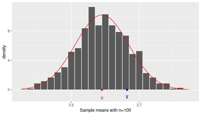
FIGURE 8.1: The distribution of the sample mean.
The histogram in Figure 8.1 is drawn using many sample mean weights from random samples of size \(n=100\).
The added red smooth curve is the density curve for the normal distribution with the appropriate expected value and standard error calculated from the sample distribution.
The red dot represents the population mean \(\mu\), the unknown parameter we are trying to estimate. The blue right is the sample mean \(\overline{x} = 3.682\) from the random sample stored in almonds_sample_100.
In real-life applications, a sample mean is taken from a sample, but the distribution of the population and the population mean are unknown, so the location of the blue dot with respect to the red dot is also unknown. However, if we construct an interval centered on the blue dot, as long as it is wide enough the interval will contain the red dot. To understand this better, we need to learn a few additional properties of the normal distribution.
8.1.2 The normal distribution
A random variable can take on different values. When those values can be represented by one or more intervals, the likelihood of those values can be expressed graphically by a density curve on a Cartesian coordinate system in two dimensions. The horizontal axis (X-axis) represents the values that the random variable can take and the height of density curve (Y-axis) provides a graphical representation of the likelihood of those values; the higher the curve the more likely those values are. In addition, the total area under a density curve is always equal to 1. The set of values a random variable can take alongside their likelihood is what we call the distribution of a random variable.
The normal distribution is the distribution of a special type of random variable. Its density curve has a distinctive bell shape, and it is fully defined by two values: (1) the mean or expected value of the random variable, \(\mu\), which is located on the X-axis at the center of the density curve (its highest point), and (2) the standard deviation, \(\sigma\), which reflects the dispersion of the random variable; the greater the standard deviation is the wider the curve appears. In Figure 8.2, we plot the density curves of three random variables, all following normal distributions:
- The solid line represents a normal distribution with \(\mu = 5\) & \(\sigma = 2\).
- The dotted line represents a normal distribution with \(\mu = 5\) & \(\sigma = 5\).
- The dashed line represents a normal distribution with \(\mu = 15\) & \(\sigma = 2\).
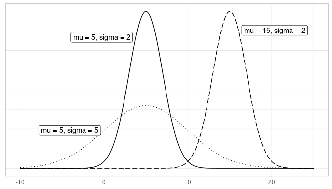
FIGURE 8.2: Three normal distributions.
A random variable that follows a normal distribution can take any values in the real line, but those values (on the X-axis) that correspond to the peak of the density curve are more likely than those corresponding to the tails. The density curve drawn with a solid line has the same mean as the one drawn with a dotted line, \(\mu = 5\), but the former exhibits less dispersion, measured by the standard deviation \(\sigma =2\), than the latter, \(\sigma = 5\). Since the total area under any density curve is equal to 1, the wider curve has to be shorter in height to preserve this property. On the other hand, the density curve drawn with a solid line has the same standard deviation as the one drawn with a dashed line, \(\sigma = 2\), but the latter has a greater mean, \(\mu = 15\), than the former, \(\mu = 5\), so they do look the same but the latter is centered farther to the right on the X-axis than the former.
The standard normal distribution
A special normal distribution has mean \(\mu\) = 0 and standard deviation \(\sigma\) = 1. It is called the standard normal distribution, and it is represented by a density curve called the \(z\)-curve. If a random variable \(Z\) follows the standard normal distribution, a realization of this random variable is called a standard value or \(z\)-value. The \(z\)-value also represents the number of standard deviations above the mean, if positive, or below the mean, if negative. For example, if \(z=5\), the value observed represents a realization of the random variable \(Z\) that is five standard deviations above the mean, \(\mu = 0\).
Linear transformations of random variables that follow the normal distribution
A linear transformation of a random variable transforms the original variable into a new random variable by adding, subtracting, multiplying, or dividing constants to the original values. The resulting random variable could have a different mean and standard deviation. The most interesting transformation is turning a random variable into another with \(\mu = 0\) and \(\sigma = 1\). When this happens we say that the random variable has been standardized.
A property of the normal distribution is that any linear transformation of a random variable that follows the normal distribution results in a new random variable that also follows a normal distribution, potentially with different mean and standard deviation. In particular, we can turn any random variable that follows the normal distribution into a random variable that follows the standard normal distribution. For example, if a value \(x = 11\) comes from a normal distribution with mean \(\mu =5\) and standard deviation \(\sigma = 2\), the \(z\)-value
\[z = \frac{x - \mu}{\sigma} = \frac{11 - 5}{2} = 3\] is the corresponding value in a standard normal curve. Moreover, we have determined that \(x = 11\) for this example is precisely \(3\) standard deviations above the mean.
Finding probabilities under a density curve
When a random variable can be represented by a density curve, the probability that the random variable takes a value in any given interval (on the X-axis) is equal to the area under the density curve for that interval. If we know the equation that represents the density curve, we could use the mathematical technique from calculus known as integration to determine this area. In the case of the normal curve, the integral for any interval does not have a close-form solution, and the solution is calculated using numerical approximations.
Please review Appendix A online where we provide R code to work with different areas, probabilities, and values under a normal density curve. Here, we place focus on the insights of specific values and areas without dedicating time to those calculations.
We assume that a random variable \(Z\) follows a standard normal distribution. We would like to know how likely it is for this random variable to take a value that is within one standard deviation from the mean. Equivalently, what is the probability that the observed value \(z\) (in the X-axis) is between -1 and 1 as shown in Figure 8.3?
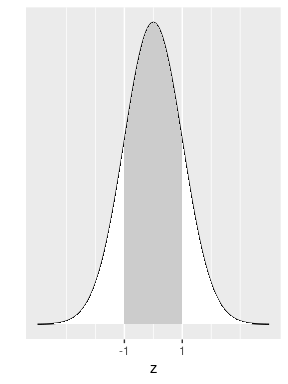
FIGURE 8.3: Normal area within one standard deviation.
Calculations show that this area is 0.6827 (68.27%) of the total area under the curve. This is equivalent to saying that the probability of getting a value between \(-1\) and 1 on a standard normal is 68.27%. This also means that if a random variable representing an experiment follows a normal distribution, the probability that the outcome of this experiment is within one standard deviation from the mean is 68.27%. Similarly, the area under the standard normal density curve between -2 and 2 is shown in Figure 8.4.
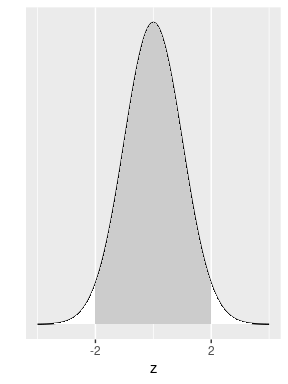
FIGURE 8.4: Normal area within two standard deviations.
Calculations show that this area is equal to 0.9545 or 95.45%. If a random variable representing an experiment follows a normal distribution, the probability that the outcome of this experiment is within two standard deviations from the mean is 95.45%. It is also common practice to use the exact number of standard deviations that correspond to an area around the mean exactly equal to 95% (instead of 95.45%). Please see Appendix A online to produce these or other calculations in R. The result is that the area under the density curve around the mean that is exactly equal to 0.95, or 95%, is the area within 1.96 standard deviation from the mean. Remember this number as it will be used a few times in later sections.
In summary, if the possible outcomes of an experiment can be expressed as a random variable that follows the normal distribution, the probability of getting a result that is within one standard deviation from the mean is about 68.27%, within 2 standard deviations form the mean is 95.45%, within 1.96 standard deviations from the mean is 95%, and within 3 standard deviations from the mean is about 99.73%, to name a few. Spend a few moments grasping this idea; observe, for example, that it is almost impossible to observe an outcome represented by a number that is five standard deviations above the mean as the chances of that happening are near zero. We are now ready to return to our main goal: how to find an interval estimate of the population mean based on a single sample.
Learning check
(LC8.3) What does the population mean (\(\mu\)) represent in the context of the almond activity?
- A. The average weight of 100 randomly sampled almonds.
- B. The weight of the heaviest almond in the bowl.
- C. The average weight of all 5,000 almonds in the bowl.
- D. The total weight of all almonds in the bowl.
(LC8.4) Which of the following statements best describes the population standard deviation (\(\sigma\)) in the almond activity?
- A. It measures the average difference between each almond’s weight and the sample mean weight.
- B. It measures the average difference between each almond’s weight and the population mean weight.
- C. It is equal to the square root of the sample variance.
- D. It is always smaller than the population mean.
(LC8.5) Why do we use the sample mean to estimate the population mean in the almond activity?
- A. Because the sample mean is always larger than the population mean.
- B. Because the sample mean is a good estimator of the population mean due to its unbiasedness.
- C. Because the sample mean requires less computational effort than the population mean.
- D. Because the sample mean eliminates all sampling variation.
8.1.3 The confidence interval
We continue using the example where we try to estimate the population mean weight of almonds with a random sample of 100 almonds. We showed in Chapter 7 that the sampling distribution of the sample mean weight of almonds approximates a normal distribution with expected value equal to the population mean weight of almonds and a standard error equal to
\[SE(\bar x) = \frac{\sigma}{\sqrt {100}}.\] In Subsection 8.1.1 we showed that for the population of almonds, \(\mu =3.645\) grams and \(\sigma = 0.392\), so the standard error for the sampling distribution is
\[SE(\bar x) = \frac{\sigma}{\sqrt{100}} = \frac{0.392}{\sqrt{100}} = 0.039\] grams. In Figure 8.5 we plot the density curve for this distribution using these values.
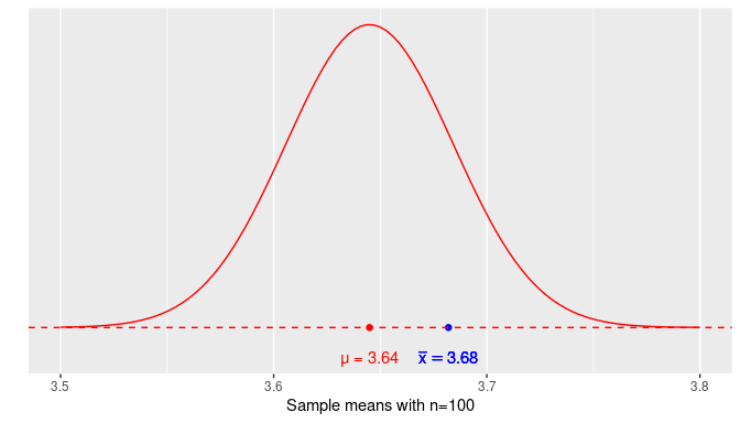
FIGURE 8.5: Normal density curve for the sample mean weight of almonds.
The horizontal axis (X-axis) represents the sample means that we can determine from all the possible random samples of 100 almonds. The red dot represents the expected value of the sampling distribution, \(\mu = 3.64\), located on the X-axis at the center of the distribution. The density curve’s height can be thought of as how likely those sample means are to be observed. For example, it is more likely to get a random sample with a sample mean around \(3.645\) grams (which corresponds to the highest point of the curve) than it is to get a sample with a sample mean of around \(3.5\) grams, since the curve’s height is almost zero at that value. The blue dot is the sample mean from our sample of 100 almonds, \(\overline{x} = 3.682\) grams. It is located 0.037 grams above the population mean weight. How far is 0.037 grams? It is helpful to express this distance in standardized values:
\[\frac{3.682 - 3.645}{0.039} = 0.945\]
so 0.037 more grams is about 0.945 standard errors above the population mean.
In real-life situations, the population mean, \(\mu\), is unknown so the distance from the sample mean to \(\mu\) is also unknown. On the other hand, the sampling distribution of the sample mean follows a normal distribution. Based on our earlier discussion about areas under the normal curve, there is a 95% chance that the value observed is within 1.96 standard deviations from the mean. In the context of our problem, there is a 95% chance that the sample mean weight is within 1.96 standard errors from the population mean weight. As shown earlier, the sample mean calculated in our example was 0.945 standard errors above the population mean, well within the reasonable range.
Think about this result. If we were to take a different random sample of 100 almonds, the sample mean will likely be different, but you still have a 95% chance that the new sample mean will be within 1.96 standard errors from the population mean.
We can finally construct an interval estimate that takes advantage of this configuration. We center our interval at the sample mean observed and then extend to each side the magnitude equivalent to 1.96 standard errors. The lower and upper bounds of this interval are:
\[\begin{aligned}\left(\overline{x} - 1.96 \frac{\sigma}{\sqrt{n}},\quad \overline{x} + 1.96 \frac{\sigma}{\sqrt{n}}\right) &= \left(3.682 - 1.96 \cdot \frac{0.392}{\sqrt{100}},\quad 3.682 + 1.96 \cdot \frac{0.392}{\sqrt{100}}\right)\\ &= (3.605, 3.759)\end{aligned}\]
Here is R code that can be used to calculate these lower and upper bounds:
almonds_sample_100 |>
  summarize(
    sample_mean = mean(weight),
    lower_bound = mean(weight) - 1.96 * sigma / sqrt(length(weight)),
    upper_bound = mean(weight) + 1.96 * sigma / sqrt(length(weight))
  )
# A tibble: 1 × 4
replicate sample_mean lower_bound upper_bound
<int> <dbl> <dbl> <dbl>
1 1 3.682 3.60515 3.75885The functions mean() and length() find the sample mean weight and sample size, respectively, from the sample of almonds’ weights in almonds_sample_100. The number 1.96 corresponds to the number of standard errors needed to get a 95% area under the normal distribution and the population standard deviation sigma of 0.392 was found in Subsection 8.1.1. Figure 8.6 shows this interval as a horizontal blue line. Observe how the population mean \(\mu\) is part of this interval.
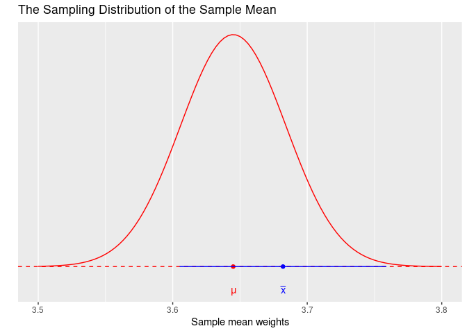
FIGURE 8.6: Is the population mean in the interval?
Since 1.96 standard errors were used on the construction of this interval, we call this a 95% confidence interval. A confidence interval can be viewed as an interval estimator of the population mean. Compare an interval estimator with the sample mean that is a point estimator. The latter estimates the parameter with a single number, the former provides an entire interval to account for the location of the parameter. An apt analogy involves fishing. Imagine that there is a single fish swimming in murky water. The fish is not visible but its movement produces ripples on the surface that can provide some limited information about the fish’s location. To capture the fish, one could use a spear or a net. Because the information is limited, throwing the spear at the ripples may capture the fish but likely will miss it.
Throwing a net around the ripples, on the other hand, may give a much higher likelihood of capturing the fish. Using the sample mean only to estimate the population mean is like throwing a spear at the ripples in the hopes of capturing the fish. Constructing a confidence interval that may include the population mean is like throwing a net to surround the ripples. Keep this analogy in mind, as we will revisit it in later sections.
Learning check
(LC8.6) How is the standard error of the sample mean weight of almonds calculated in the context of this example?
- A. By dividing the sample mean by the population standard deviation.
- B. By dividing the population standard deviation by the square root of the sample size.
- C. By multiplying the sample mean by the square root of the sample size.
- D. By dividing the population mean by the sample size.
(LC8.7) What does a 95% confidence interval represent in the context of the almond weight estimation?
- A. There is a 95% chance that the sample mean is within 1.96 standard deviations from the population mean.
- B. The interval will contain 95% of the almond weights from the sample.
- C. There is a 95% chance that the population mean falls within 1.96 standard errors from the sample mean.
- D. The sample mean is exactly equal to the population mean 95% of the time.
8.1.4 The t distribution
Recall that due to the Central Limit Theorem, the sampling distribution of the sample mean was approximately normal with mean equal to the population mean \(\mu\) and standard deviation given by the standard error \(SE(\overline X) = \sigma/\sqrt{n}\). We can standardize this for any sample mean \(\overline{x}\) such that
\[z = \frac{\overline{x} - \mu}{\sigma/\sqrt{n}}\]
is the corresponding value of the standard normal distribution.
In the construction of the interval in Figure 8.6 we have assumed the population standard deviation, \(\sigma\), was known, and therefore we have used it to find the confidence interval. Nevertheless, in real-life applications, the population standard deviation is also unknown. Instead, we use the sample standard deviation, \(s\), from the sample we have, as an estimator of the population standard deviation \(\sigma\). Our estimated standard error is given by
\[\widehat{SE}(\overline X) = \frac{s}{\sqrt n}.\]
When using the sample standard deviation to estimate the standard error, we are introducing additional uncertainty in our model. For example, if we try to standardize this value, we get
\[t = \frac{\overline{x} - \mu}{s/\sqrt{n}}.\]
Because we are using the sample standard deviation in this equation and since the sample standard deviation changes from sample to sample, the additional uncertainty makes the values \(t\) no longer normal. Instead they follow a new distribution called the \(t\) distribution.
The \(t\) distribution is similar to the standard normal; its density curve is also bell-shaped, and it is symmetric around zero, but the tails of the \(t\) distribution are a little thicker than those of the standard normal. In addition, the \(t\) distribution requires one additional parameter, the degrees of freedom. For sample mean problems, the degrees of freedom needed are exactly \(n-1\), the size of the sample minus one. Figure 8.7 shows the density curves of
- the standard normal density curve, in black,
- a \(t\) density curve for a t distribution with 2 degrees of freedom, in dotted blue, and
- a \(t\) density curve for a t distribution with 10 degrees of freedom, in dashed red.
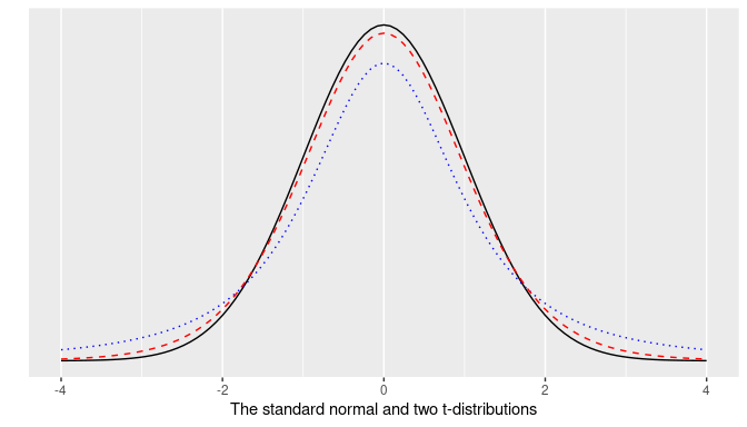
FIGURE 8.7: The standard normal and two t-distributions.
Observe how the \(t\) density curve in dashed red (\(t\) with 10 degrees of freedom) gets closer to the standard normal density curve, or \(z\)-curve, in solid black, than the \(t\) curve in dotted blue (\(t\) with 2 degrees of freedom). The greater the number of degrees of freedom, the closer the \(t\) density curve is from the \(z\) curve. This change makes our calculations slightly different.
Please see Appendix A online for calculations of probabilities for \(t\) density curves with different degrees of freedom. Using that knowledge, the calculation for our specific example shows that 95% of the sample means are within 1.98 standard errors from the population mean weight. The number of standard errors needed is not that different from before, 1.98 versus 1.96, because the degrees of freedom are fairly large.
Using this information, we can construct the 95% confidence interval based entirely on our sample information and using the sample mean and sample standard deviation. We calculate those values again for almonds_sample_100:
# A tibble: 1 × 3
  replicate sample_mean sample_sd
      <int>       <dbl>     <dbl>
1         1       3.682  0.362199
Observe that the sample standard deviation is \(s = 0.362\) which is not that different from the population standard deviation of \(\sigma = 0.392\). We again center the confidence interval at the observed sample mean but now extend the interval by 1.98 standard errors to each side. The lower and upper bounds of this confidence interval are:
\[ \begin{aligned} \left(\overline{x} - 1.98 \frac{s}{\sqrt{n}},\quad \overline{x} + 1.98 \frac{s}{\sqrt{n}}\right) &= \left(3.682 - 1.98 \cdot \frac{0.362}{\sqrt{100}}, 3.682 + 1.98 \cdot \frac{0.362}{\sqrt{100}}\right) \\ &= (3.498, 3.846)) \end{aligned} \]
We can also compute these lower and upper bounds:
almonds_sample_100 |>
  summarize(sample_mean = mean(weight), sample_sd = sd(weight),
            lower_bound = mean(weight) - 1.98*sd(weight)/sqrt(length(weight)),
            upper_bound = mean(weight) + 1.98*sd(weight)/sqrt(length(weight)))
# A tibble: 1 × 5
replicate sample_mean sample_sd lower_bound upper_bound
<int> <dbl> <dbl> <dbl> <dbl>
1 1 3.682 0.362199 3.61028 3.75372The confidence interval computed here, using the sample standard deviation and a \(t\) distribution, is almost the same as the one attained using the population standard deviation and the standard normal distribution, the difference is about 0.005 units for the upper and lower bound. This happens because with a sample size of 100, the \(t\)-curve and \(z\)-curve are almost identical and also because the sample standard deviation was very similar to the population standard deviation. This does not have to be always the case and occasionally we can observe greater differences; but, in general, the results are fairly similar.
More importantly, the confidence interval constructed here contains the population mean of \(\mu = 3.645\), which is the result we needed. Recall that a confidence interval is an interval estimate of the parameter of interest, the population mean weight of almonds. We can summarize the results so far:
- If the size used for your random sample is large enough, the sampling distribution of the sample mean follows, approximately, the normal distribution.
- Using the sample mean observed and the standard error of the sampling distribution, we can construct 95% confidence intervals for the population mean. The formula for these intervals (where \(n\) is the sample size used) is given by
\[\left(\overline{x} - 1.96 \frac{\sigma}{\sqrt{n}},\quad \overline{x} + 1.96 \frac{\sigma}{\sqrt{n}}\right).\]
- When the population standard deviation is unknown (which is almost always the case), the sample standard deviation is used to estimate the standard error. This produces additional variability and the standardized values follow a \(t\) distribution with \(n-1\) degrees of freedom. The formula for 95% confidence intervals when the sample size is \(n=100\) is given by
\[\left(\overline{x} - 1.98 \frac{s}{\sqrt{100}},\quad \overline{x} + 1.98 \frac{s}{\sqrt{100}}\right).\]
- The method to construct 95% confidence intervals guarantees that in the long-run for 95% of the possible samples, the intervals determined will include the population mean. It also guarantees that 5% of the possible samples will lead to intervals that do not include the population mean.
- As we have constructed intervals with a 95% level of confidence, we can construct intervals with any level of confidence. The only change in the equations will be the number of standard errors needed.
8.1.5 Interpreting confidence intervals
We have used the sample almonds_sample_100, constructed a 95% confidence interval for the population mean weight of almonds, and showed that the interval contained this population. This result is not surprising as we expect intervals such as this to include the population mean for 95% of the possible random samples. We repeat this interval construction for many random samples. Figure 8.8 presents the results for one hundred 95% confidence intervals.
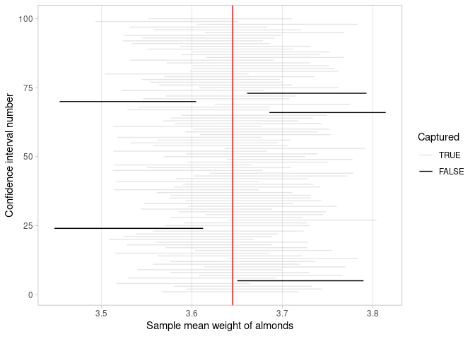
FIGURE 8.8: One hundred 95% confidence intervals and whether the population mean is captured in each.
Note that each interval was built using a different random sample. The red vertical line is drawn at the location of the population mean weight, \(\mu = 3.645\). The horizontal lines represent the one hundred 95% confidence intervals found. The gray confidence intervals cross the red vertical line so they contain the population mean. The black confidence intervals do not.
This result motivates the meaning of a 95% confidence interval: If you could construct intervals using the procedure described earlier for every possible random sample, then 95% of these intervals will include the population mean and 5% of them will not.
Of course, in most situations, it would be impractical or impossible to take every possible random sample. Still, for a large number of random samples, this result is approximately correct. In Figure 8.8, for example, 5 out of 100 confidence intervals do not include the population mean, and 95% do. It won’t always match up perfectly like this, but the proportions should match pretty close to the confidence level chosen.
The term “95% confidence” invites us to think we are talking about probabilities or chances. Indeed we are, but in a subtle way. Before a random sample has been procured, there is a 95% chance that when a confidence interval is constructed using the prospective random sample, this interval will contain the population mean. The moment a random sample has been attained, the interval constructed either contains the population mean or it does not; with certainty, there is no longer a chance involved. This is true even if we do not know what the population mean is. So the 95% confidence refers to the method or process to be used on a prospective sample. We are confident that if we follow the process to construct the interval, 95% of the time the random sample attained will lead us to produce an interval that contains the population mean.
On the other hand, it would be improper to say that… “there is a 95% chance that the confidence interval contains the population mean.” Looking at Figure 8.8, each of the confidence intervals either does or does not contain \(\mu\). Once the confidence interval is determined, either the population mean is included or not.
In the literature, this explanation has been encapsulated in a short-hand version: we are 95% confident that the interval contains the population parameter. For example, in Subsection 8.1.4 the 95% confidence interval for the population mean weight of almonds was (3.498, 3.846), and we would say: “We are 95% confident that the population mean weight of almonds is between 3.498 and 3.846 grams.”
It is perfectly acceptable to use the short-hand statement, but always remember that the 95% confidence refers to the process, or method, and can be thought of as a chance or probability only before the random sample has been acquired. To further ensure that the probability-type of language is not misused, quotation marks are sometimes put around “95% confident” to emphasize that it is a short-hand version of the more accurate explanation.
Learning check
(LC8.8) Why does the \(t\) distribution have thicker tails compared to the standard normal distribution?
- A. Because the sample mean is considered more likely to match the population mean closely.
- B. Because the \(t\) distribution is designed to work when the data does not follow a normal distribution.
- C. Because it assumes that the sample size is always smaller when applying the \(t\) distribution.
- D. Because it accounts for the extra uncertainty that comes from using the sample standard deviation instead of the population standard deviation.
(LC8.9) What is the effect of increasing the degrees of freedom on the \(t\) distribution?
- A. The tails of the distribution become thicker.
- B. The tails of the distribution become thinner.
- C. The distribution does not change with degrees of freedom.
- D. The distribution becomes skewed to the right.
Understanding the width of a confidence interval
A confidence interval is an estimator of a population parameter. In the case of the almonds’ bowl we constructed a confidence interval for the population mean. The equation to construct a 95% confidence interval was
\[\left(\overline{x} - 1.96 \frac{\sigma}{\sqrt{n}}, \overline{x} + 1.96 \frac{\sigma}{\sqrt{n}}\right)\] Observe that the confidence interval is centered at the sample mean and it extends to each side 1.96 standard errors \(1.96\cdot \sigma / \sqrt{n}\). This quantity is exactly half the width of your confidence interval, and it is called the margin of error. The value of the population standard deviation, \(\sigma\), is beyond our control, as it is determined by the distribution of the experiment or phenomenon studied. The sample mean, \(\overline{x}\), is a result that depends on your random sample exclusively. On the other hand, the number 1.96 and the sample size, \(n\), are values that can be changed by the researcher or practitioner. They play an important role on the width of the confidence interval. We study each of them separately.
The confidence level
We mentioned earlier that the number 1.96 relates to a 95% confidence process but we did not show how to determine this value. The level of confidence is a decision of the practitioner. If you want to be more confident, say 98% or 99% confident, you just need to adjust the appropriate number of standard errors needed. We show how to determine this number, and use Figure 8.9 to illustrate this process.
- If the confidence level is 0.95 (or 95%), the area in the middle of the standard normal distribution is 0.95. This area is shaded in Figure 8.9.
- We construct \(\alpha = 1 - \text{confidence level} = 1 - 0.95 = 0.05\). Think of \(\alpha\) as the total area on both tails.
- Since the normal distribution is symmetric, the area on each tail is \(\alpha/2 = 0.05/2 = 0.025\).
- We need the exact number of standard deviations that produces the shaded area. Since the center of a standard normal density curve is zero, as shown in Figure 8.9, and the normal curve is symmetric, the number of standard deviations can be represented by \(-q\) and \(q\), the same magnitude but one positive and the other negative.
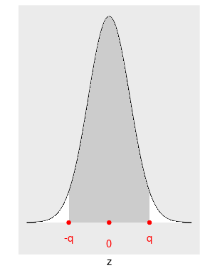
FIGURE 8.9: Normal curve with the shaded middle area being 0.95
In R, the function qnorm() finds the value of \(q\) when the area under this curve to the left of this value \(q\) is given. In our example the area to the left of \(-q\) is \(\alpha/2 = 0.05/2 = 0.025\), so
qnorm(0.025)[1] -1.96or 1.96 standard deviation below the mean. Similarly, the total area under the curve to the left of \(q\) is the total shaded area, 0.95, plus the small white area on the left tail, \(0.025\), and \(0.95 + 0.025 = 0.975\), so
qnorm(0.975)[1] 1.96That is the reason we use 1.96 standard deviation when calculating 95% confidence intervals. What if we want to retrieve a 90% confidence interval? We follow the same procedure:
- The confidence level is 0.90.
- \(\alpha = 1 - \text{confidence level} = 1 - 0.90 = 0.10\).
- The area on each tail is \(\alpha/2 = 0.10/2 = 0.05\).
- The area needed to find \(q\) is \(0.90+0.05 = 0.95\).
qnorm(0.95)[1] 1.65If we want to determine a 90% confidence interval, we need to use 1.645 standard errors in our calculations. We can update the R code to calculate the lower and upper bounds of a 90% confidence interval:
almonds_sample_100 |>
  summarize(sample_mean = mean(weight),
            lower_bound = mean(weight) - qnorm(0.95)*sigma/sqrt(length(weight)),
            upper_bound = mean(weight) + qnorm(0.95)*sigma/sqrt(length(weight)))
# A tibble: 1 × 4
replicate sample_mean lower_bound upper_bound
<int> <dbl> <dbl> <dbl>
1 1 3.682 3.61751 3.74649Let’s do one more. If we want an 80% confidence interval, \(1 - 0.8 = 0.2\), \(0.2/2 = 0.1\), and \(0.8+0.1 = 0.9\), so
qnorm(0.9)[1] 1.28When you want to calculate an 80%, 90%, or 95% confidence interval, you need to construct your interval using 1.282, 1.645, or 1.96 standard errors, respectively. The more confident you want to be, the larger the number of standard errors you need to use, and the wider your confidence interval becomes. But a confidence interval is an estimator of the population mean, the narrower it is, the more useful it is for practical reasons. So there is a trade-off between the width of a confidence interval and the confidence you want to have.
The sample size
As we studied changes to the confidence level, we can determine how big is the random sample used. The margin of error for a 95% confidence interval is
\[1.96\cdot \frac{\sigma}{\sqrt{n}}.\]
If the sample size increases, the margin of error decreases proportional to the square root of the sample size. For example, if we secure a random sample of size 25, \(1/\sqrt{25} = 0.2\), and if we draw a sample of size 100, \(1/\sqrt{100} = 0.1\). By choosing a larger sample size, four times larger, we produce a confidence interval that is half the width. This result is worth considering.
A confidence interval is an estimator of the parameter of interest, such as the population mean weight of almonds. Ideally, we would like to build a confidence interval with a high level of confidence, for example, 95% confidence. But we also want an interval that is narrow enough to provide useful information. For example, assume we get the following 95% confidence intervals for the population mean weight of almonds:
- between 2 and 4 grams, or
- between 3.51 and 3.64 grams, or
- between 3.539 and 3.545 grams.
The first interval does not seem useful at all, the second works better, and the third is tremendously accurate, as we are 95% confident that the population mean is within 0.006 grams. Obviously, we always prefer narrower intervals, but there are trade-offs we need to consider. We always prefer high levels of confidence, but the more confident we want to be the wider the interval will be. In addition, the larger the random sample used, the narrower the confidence interval will be. Using a large sample is always a preferred choice, but the trade-offs are often external; collecting large samples could be expensive and time-consuming. The construction of confidence intervals needs to take into account all these considerations.
We have concluded the theory-based approach to construct confidence intervals. In the next section we explore a completely different approach to construct confidence intervals and in later sections we will make comparisons of these methods.
8.2 Estimation with the bootstrap
In 1979, Brad Efron published an article introducing a method called the bootstrap (Efron 1979) that is next summarized. A random sample of size \(n\) is taken from the population. This sample is used to find another sample, with replacement, also of size \(n\). This is called resampling with replacement and the resulting sample is called a bootstrap sample. For example, if the original sample is \(\{4,2,5,4,1,3,7,4,6,1\}\), one particular bootstrap sample could be \(\{6, 4, 7, 4, 2, 7, 2, 5, 4, 1\}.\) Observe that the number 7 appears once in the original sample, but twice in the bootstrap sample; similarly, the number 3 in the original sample does not appear in the bootstrap sample. This is not uncommon for a bootstrap sample, some of the numbers in the original sample are repeated and others are not included.
The basic idea of the bootstrap is to gain a large number of bootstrap samples, all drawn from the same original sample. Then, we use all these bootstrap samples to find estimates of population parameters, standard errors, or even the density curve of the population. Using them we can construct confidence intervals, perform hypothesis testing, and other inferential methods.
This method takes advantage of the large number of bootstrap samples that can be determined. In several respects, this exercise is not different from the sampling distribution explained in Chapter 7. The only difference, albeit an important one, is that we are not sampling from the population, we are sampling from the original sample. How many different bootstrap samples could we get from a single sample? A very large number, actually. If the original sample has 10 numbers, as the one shown above, each possible bootstrap sample of size 10 is determined by sampling 10 times with replacement, so the total number of bootstrap samples is \(10^{10}\) or 10 billion different bootstrap samples. If the original sample has 20 numbers, the number of bootstrap samples is \(20^{20}\), a number greater than the total number of stars in the universe. Even with modern powerful computers, it would be an onerous task to calculate every possible bootstrap sample. Instead, a thousand or so bootstrap samples are retrieved, similar to the simulations performed in Chapter 7, and this number is often large enough to provide useful results.
Since Efron (Efron 1979) proposed the bootstrap, the statistical community embraced this method. During the 1980s and 1990s, many theoretical and empirical results were presented showing the strength of bootstrap methods. As an illustration, Efron (Efron 1979), Hall (Hall 1986), Efron and Tibshirani(Efron and Tibshirani 1986), and Hall (Hall 1988) showed that bootstrapping was at least as good if not better than existent methods, when the goal was to estimate the standard error of an estimator or find the confidence intervals of a parameter. Modifications were proposed to improve the algorithm in situations where the basic method was not producing accurate results. With the continuous improvement of computing power and speed, and the advantages of having ready-to-use statistical software for its implementation, the use of the bootstrap has become more and more popular in many fields.
As an illustration, if we are interested in the mean of the population, \(\mu\), and we have collected one random sample, we can gain a large number of bootstrap samples from this original sample, use them to calculate sample means, order the sample means from smallest to largest, and choose the interval that contains the middle 95% of these sample means. This will be the simplest way to find a confidence interval based on the bootstrap. In the next few subsections, we explore how to incorporate this and similar methods to construct confidence intervals.
8.2.1 Bootstrap samples: revisiting the almond activity
To study and understand the behavior of bootstrap samples, we return to our example of the chocolate-covered almonds in a bowl. Recall that the bowl is considered the population of almonds, and we are interested in estimating the population mean weight of almonds.
As we did before, we only have access to a single random sample. In this section, we use the data frame almonds_sample_100, a random sample of 100 almonds taken earlier. We call this the original sample, and it is used in this section to create the bootstrap samples.
The first 10 rows are shown:
almonds_sample_100# A tibble: 100 × 3
# Groups: replicate [1]
replicate ID weight
<int> <int> <dbl>
1 1 166 4.2
2 1 1215 4.2
3 1 1899 3.9
4 1 1912 3.8
5 1 4637 3.3
6 1 511 3.5
7 1 127 4
8 1 4419 3.5
9 1 4729 4.2
10 1 2574 4.1
# ℹ 90 more rowsConstructing a bootstrap sample: resampling once
We start by constructing one bootstrap sample of 100 almonds from the original sample of 100 almonds. These are the steps needed to perform this task manually:
Step 1: Place the original sample of 100 almonds into a bag or hat.
Step 2: Mix the bag contents, draw one almond, weigh it, and record the weight as seen in Figure 8.10.
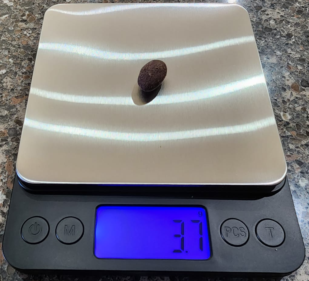
FIGURE 8.10: Step 2: Weighing one almond at random.
Step 3: Put the almond back into the bag! In other words, replace it as seen in Figure 8.11.
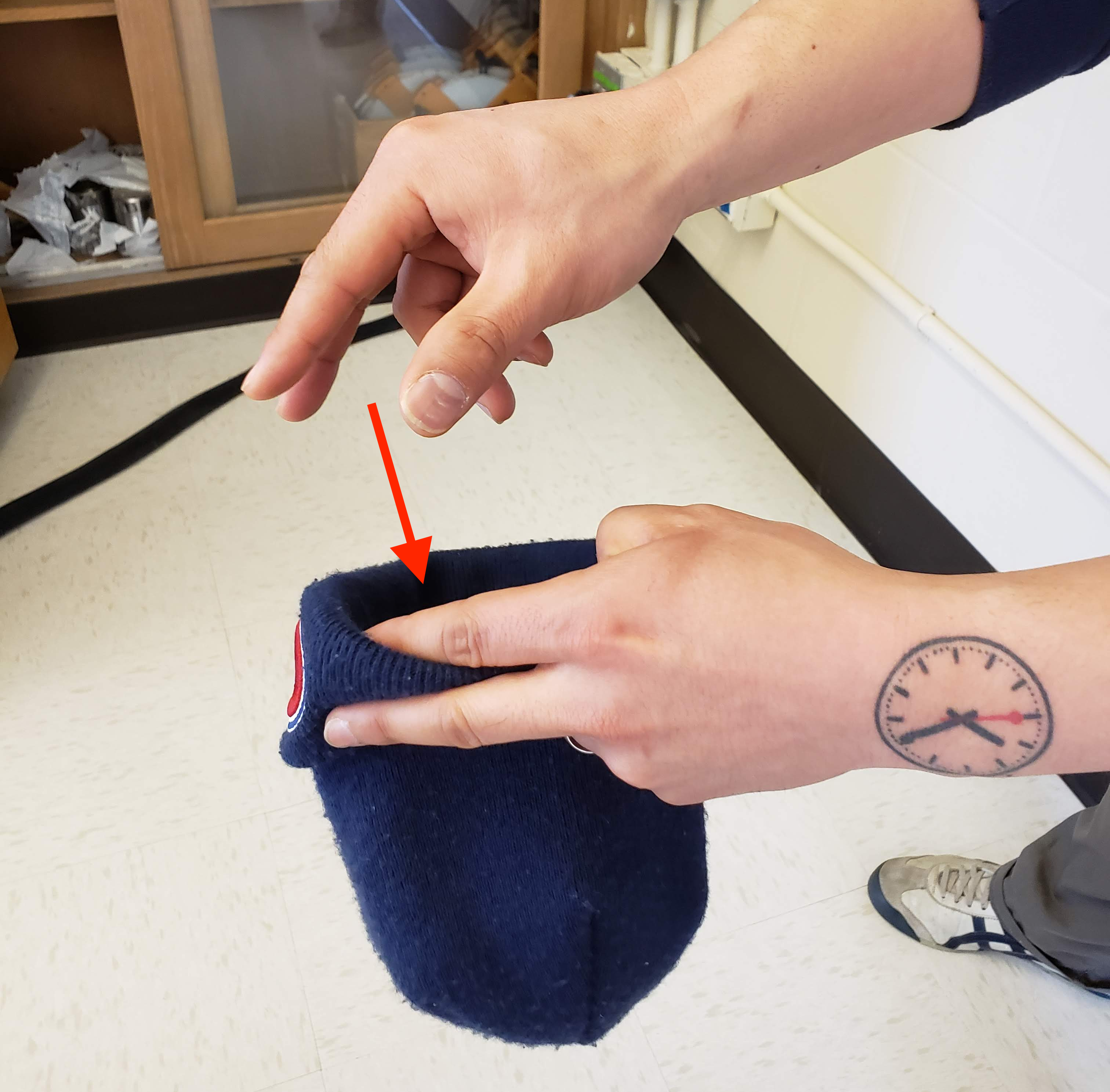
FIGURE 8.11: Step 3: Replacing almond.
Step 4: Repeat Steps 2 and 3 a total of 99 more times, resulting in 100 weights.
These steps describe resampling with replacement, and the resulting sample is called a bootstrap sample. This procedure results in some almonds being chosen more than once and other almonds not being chosen at all. Resampling with replacement induces sampling variation, so every bootstrap sample can be different than any other.
This activity can be performed manually following the steps described above. We can also take advantage of the R code we have introduced in Chapter 7 and do this virtually.
The data frame almonds_sample_100 contains the random sample of almonds taken from the population. We show selected rows from this sample.
# A tibble: 100 × 2
      ID weight
   <int>  <dbl>
 1   166    4.2
 2  1215    4.2
 3  1899    3.9
 4  1912    3.8
 5  4637    3.3
 6   511    3.5
 7   127    4
 8  4419    3.5
 9  4729    4.2
10  2574    4.1
# ℹ 90 more rows
We use ungroup() and select to eliminate the variable replicate from the almonds_sample_100 as this variable may create clutter when resampling. We can now create a bootstrap sample also of size 100 by resampling with replacement once.
boot_sample <- almonds_sample_100 |>
  rep_sample_n(size = 100, replace = TRUE, reps = 1)
We have used this type of R syntax many times in Chapter 7.
We first select the data frame almonds_sample_100 that contains the almonds’ weights in the original sample.
We then perform resampling with replacement once: we resample by using rep_sample_n(), a sample of size 100 by setting size = 100, with replacement by adding the argument replace = TRUE, and one time by setting reps = 1.
The object boot_sample is a bootstrap sample of 100 almonds’ weights gained from the original sample of 100 almonds’ weights. We show the first ten rows of boot_sample:
boot_sample# A tibble: 100 × 3
# Groups: replicate [1]
replicate ID weight
<int> <int> <dbl>
1 1 2105 3.1
2 1 4529 3.8
3 1 1146 4.2
4 1 2993 3.2
5 1 1535 3.2
6 1 2294 3.7
7 1 438 3.8
8 1 4419 3.5
9 1 1674 3.5
10 1 1146 4.2
# ℹ 90 more rowsWe can also study some of the characteristics of this bootstrap sample, such as its sample mean:
# A tibble: 1 × 2
  replicate mean_weight
      <int>       <dbl>
1         1       3.702
By using summarize() and mean() on the bootstrap sample boot_sample, we determine that the mean weight is 3.702 grams. Recall that the sample mean of the original sample was found in the previous subsection as 3.682. So, the sample mean of the bootstrap sample is different than the sample mean of the original sample. This variation is induced by resampling with replacement, the method for finding the bootstrap sample. We can also compare the histogram of weights for the bootstrap sample with the histogram of weights for the original sample.
ggplot(boot_sample, aes(x = weight)) +
  geom_histogram(binwidth = 0.1, color = "white") +
  labs(title = "Resample of 100 weights")
ggplot(almonds_sample_100, aes(x = weight)) +
  geom_histogram(binwidth = 0.1, color = "white") +
  labs(title = "Original sample of 100 weights")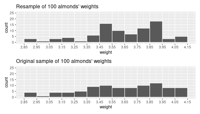
FIGURE 8.12: Comparing weight in the resampled boot_sample with the original sample almonds_sample_100.
Observe in Figure 8.12 that while the general shapes of both distributions of weights are roughly similar, they are not identical.
This is the typical behavior of bootstrap samples. They are samples that have been determined from the original sample, but because replacement is used before each new observation is attained, some values often appear more than once while others often do not appear at all.
Many bootstrap samples: resampling multiple times
In this subsection, we take full advantage of resampling with replacement by taking many bootstrap samples and study relevant information, such as the variability of their sample means. We can start by using the R syntax we used before, this time for 35 replications.
bootstrap_samples_35 <- almonds_sample_100 |>
  rep_sample_n(size = 100, replace = TRUE, reps = 35)
bootstrap_samples_35
# A tibble: 3,500 × 3
# Groups: replicate [35]
replicate ID weight
<int> <int> <dbl>
1 1 1459 3.6
2 1 2972 3.4
3 1 1215 4.2
4 1 1381 3.4
5 1 1264 3.5
6 1 199 3.4
7 1 476 3.8
8 1 4806 3.7
9 1 3169 4.1
10 1 2265 3.4
# ℹ 3,490 more rowsThe syntax is the same as before, but this time we set reps = 35 to get 35 bootstrap samples.
The resulting data frame, bootstrap_samples, has 35 \(\cdot\) 100 = 3500 rows corresponding to 35 resamples of 100 almonds’ weights. Let’s now compute the resulting 35 sample means using the same dplyr code as we did in the previous section:
# A tibble: 35 × 2
   replicate mean_weight
       <int>       <dbl>
 1         1       3.68
 2         2       3.688
 3         3       3.632
 4         4       3.68
 5         5       3.679
 6         6       3.675
 7         7       3.678
 8         8       3.706
 9         9       3.643
10        10       3.68
# ℹ 25 more rows
Observe that boot_means has 35 rows, corresponding to the 35 bootstrap sample means. Furthermore, observe that the values of mean_weight vary as shown in Figure 8.13.
ggplot(boot_means, aes(x = mean_weight)) +
  geom_histogram(binwidth = 0.01, color = "white") +
  labs(x = "sample mean weight in grams")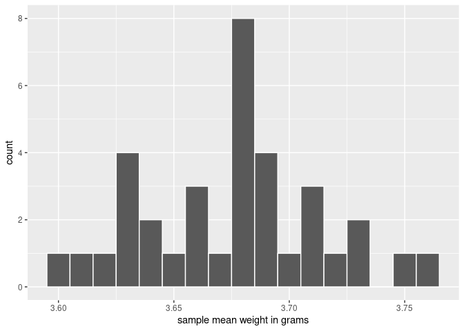
FIGURE 8.13: Distribution of 35 sample means from 35 bootstrap samples.
This histogram highlights the variation of the sample mean weights. Since we have only used 35 bootstrap samples, the histogram looks a little coarse. To improve our perception of this variation, we find 1000 bootstrap samples and their sample means:
# Retrieve 1000 bootstrap samples
bootstrap_samples <- almonds_sample_100 |>
  rep_sample_n(size = 100, replace = TRUE, reps = 1000)

# Compute sample means from the bootstrap samples
boot_means <- bootstrap_samples |>
  summarize(mean_weight = mean(weight))
We can combine these two operations into a single chain of pipe (|>) operators:
boot_means <- almonds_sample_100 |>
  rep_sample_n(size = 100, replace = TRUE, reps = 1000) |>
  summarize(mean_weight = mean(weight))
boot_means
# A tibble: 1,000 × 2
replicate mean_weight
<int> <dbl>
1 1 3.68
2 2 3.688
3 3 3.632
4 4 3.68
5 5 3.679
6 6 3.675
7 7 3.678
8 8 3.706
9 9 3.643
10 10 3.68
# ℹ 990 more rowsThe data frame boot_means contains 1000 sample mean weights. Each is calculated from a different bootstrap sample and visualized in Figure 8.14.
ggplot(boot_means, aes(x = mean_weight)) +
  geom_histogram(binwidth = 0.01, color = "white") +
  labs(x = "sample mean weight in grams")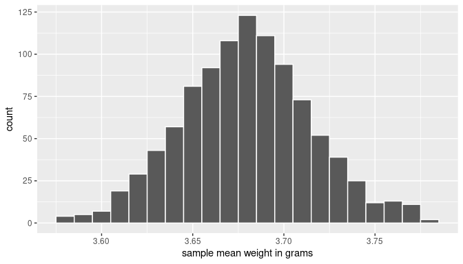
FIGURE 8.14: Histogram of 1000 bootstrap sample mean weights of almonds.
The histogram is a graphical approximation of the bootstrap distribution of the sample mean. This distribution is constructed by getting all the sample means from every bootstrap sample constructed based on the original sample. Since the total number of possible bootstraps is really large, we have not used all of them here, but 1000 of them already provides a good visual approximation.
Observe also that the bootstrap distribution itself can approximate the sampling distribution of the sample mean, a concept we studied in Chapter 7 where we took multiple samples from the population. The key difference here is that we resample from a single sample, the original sample, not from the entire population.
By inspecting the histogram in Figure 8.14, the bell-shape is apparent. We can also approximate the center and the spread of this distribution by computing the mean and the standard deviation of these 1000 bootstrap sample means:
# A tibble: 1 × 2
  mean_of_means sd_of_means
          <dbl>       <dbl>
1       3.67998   0.0356615
Everything we learned in Chapter 7 when studying the sampling distribution of the sample mean applies here. For example, observe that the mean of these bootstrap sample means is near 3.68 grams, very close to the mean of the original sample: 3.682 grams. Our intention is not to study the distribution of the bootstrap samples, but rather to use them to estimate population values, such as the population mean. In the next section, we discuss how can we use these bootstrap samples to construct confidence intervals.
Learning check
(LC8.10) What is the chief difference between a bootstrap distribution and a sampling distribution?
(LC8.11) Looking at the bootstrap distribution for the sample mean in Figure 8.14, between what two values would you say most values lie?
(LC8.12) Which of the following is true about the confidence level when constructing a confidence interval?
- A. The confidence level determines the width of the interval and affects how likely it is to contain the population parameter.
- B. The confidence level is always fixed at 95% for all statistical analyses involving confidence intervals.
- C. A higher confidence level always results in a narrower confidence interval, making it more useful for practical purposes.
- D. The confidence level is only relevant when the population standard deviation is known.
(LC8.13) How does increasing the sample size affect the width of a confidence interval for a given confidence level?
- A. It increases the width of the confidence interval, making it less precise.
- B. It has no effect on the width of the confidence interval since the confidence level is fixed.
- C. It decreases the width of the confidence interval, making it more precise by reducing the margin of error.
- D. It changes the confidence level directly, regardless of other factors.
8.2.2 Confidence intervals and the bootstrap: original workflow
The process of determining bootstrap samples and using them for estimation is called bootstrapping. We can estimate population parameters such as the mean, median, or standard deviation. We can also construct confidence intervals.
In this subsection, we focus on the latter and construct confidence intervals based on bootstrap samples. For this, we review the R syntax and workflow we have already used in previous sections and also introduce a new package: the infer package for tidy and transparent statistical inference.
Original workflow
Recall that we took bootstrap samples, then calculated the sample means from these samples. Let’s revisit the original workflow using dplyr verbs and the |> operator.
First, we use rep_sample_n() to resample from the original sample almonds_sample_100 of 5000 almonds. We set size = 100 to generate bootstrap samples of the same size as the original sample, and we resample with replacement by setting replace = TRUE. We create 1000 bootstrap samples by setting reps = 1000:
almonds_sample_100 |>
  rep_sample_n(size = 100, replace = TRUE, reps = 1000)
Second, we add another pipe followed by summarize() to compute the sample mean() weight for each replicate:
almonds_sample_100 |>
  rep_sample_n(size = 100, replace = TRUE, reps = 1000) |>
  summarize(mean_weight = mean(weight))
For this simple case, all we needed was to use the rep_sample_n() function and a dplyr verb. However, using only dplyr verbs provides us with a limited set of tools that is not ideal when working with more complicated situations. This is the reason we introduce the infer package.
8.2.3 The infer package workflow:
The infer package is an R package for statistical inference. It makes efficient use of the |> pipe operator we introduced in Section 3.1 to spell out the sequence of steps necessary to perform statistical inference in a “tidy” and transparent fashion. Just as the dplyr package provides functions with verb-like names to perform data wrangling, the infer package provides functions with intuitive verb-like names to perform statistical inference, such as constructing confidence intervals or performing hypothesis testing. We have discussed the theory-based implementation of the former in section 8.1.3 and we introduce the latter in Chapter 9.
Using the example of almonds’ weights, we introduce infer first by comparing its implementation with dplyr. Recall that to calculate a sample statistic or point estimate from a sample, such as the sample mean, when using dplyr we use summarize() and mean():
If we want to use infer instead, we use the functions specify() and calculate() as shown:
The new structure using infer seems slightly more complicated than the one using dplyr for this simple calculation. These functions will provide three chief benefits moving forward.
First, the
inferverb names better align with the overall simulation-based framework you need to understand to construct confidence intervals and to conduct hypothesis tests (in Chapter 9). We will see flowchart diagrams of this framework in the upcoming Figure 8.20 and in Chapter 9 with Figure 9.11.Second, you can transition seamlessly between confidence intervals and hypothesis testing with minimal changes to your code. This becomes apparent in Subsection 9.4.2 when we compare the
infercode for both of these inferential methods.Third, the
inferworkflow is much simpler for conducting inference when you have more than one variable. We introduce two-sample inference where the sample data is collected from two groups, such as in Section 8.4 where we study the contagiousness of yawning and in Section 9.2 where we compare the popularity of music genres. Then in Section 10.3, we see situations of inference for regression using the regression models you fit in Chapter 5.
We now illustrate the sequence of verbs necessary to construct a confidence interval for \(\mu\), the population mean weight of almonds.
1. specify variables
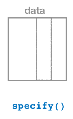
FIGURE 8.15: Diagram of the specify() verb.
As shown in Figure 8.15, the specify() function is used to choose which variables in a data frame are the focus of our statistical inference. We do this by specifying the response argument. For example, in our almonds_sample_100 data frame of the 100 almonds sampled from the bowl, the variable of interest is weight:
almonds_sample_100 |>
  specify(response = weight)
Response: weight (numeric)
# A tibble: 100 × 1
weight
<dbl>
1 4.2
2 4.2
3 3.9
4 3.8
5 3.3
6 3.5
7 4
8 3.5
9 4.2
10 4.1
# ℹ 90 more rowsNotice how the data itself does not change, but the Response: weight (numeric) meta-data does. This is similar to how the group_by() verb from dplyr doesn’t change the data, but only adds “grouping” meta-data, as we saw in Section 3.4.
We can also specify which variables are the focus of the study by introducing a formula = y ~ x in specify(). This is the same formula notation you saw in Chapters 5 and 6 on regression models: the response variable y is separated from the explanatory variable x by a ~ (“tilde”). The following use of specify() with the formula argument yields the same result seen previously:
almonds_sample_100 |>
  specify(formula = weight ~ NULL)
In the case of almonds we only have a response variable and no explanatory variable of interest. Thus, we set the x on the right-hand side of the ~ to be NULL.
In cases where inference is focused on a single sample, as it is the almonds’ weights example, either specification works. In the examples we present in later sections, the formula specification is simpler and more flexible. In particular, this comes up in the upcoming Section 8.4 on comparing two proportions and Section 10.3 on inference for regression.
2. generate replicates
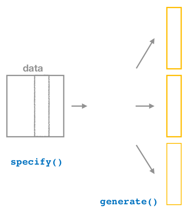
FIGURE 8.16: Diagram of generate() replicates.
After we specify() the variables of interest, we pipe the results into the generate() function to generate replicates. This is the function that produces the bootstrap samples or performs the similar resampling process a large number of times, based on the variable(s) specified previously, as shown in Figure 8.16. Recall we did this 1000 times.
The generate() function’s first argument is reps, which sets the number of replicates we would like to generate. Since we want to resample the 100 almonds in almonds_sample_100 with replacement 1000 times, we set reps = 1000.
The second argument type determines the type of computer simulation used. Setting this to type = "bootstrap" produces bootstrap samples using resampling with replacement. We present different options for type in Chapter 9.
Response: weight (numeric)
# A tibble: 100,000 × 2
# Groups:   replicate [1,000]
   replicate weight
       <int>  <dbl>
 1         1    3.6
 2         1    3.4
 3         1    4.2
 4         1    3.4
 5         1    3.5
 6         1    3.4
 7         1    3.8
 8         1    3.7
 9         1    4.1
10         1    3.4
# ℹ 99,990 more rows
Observe that the resulting data frame has 100,000 rows. This is because we have found 1000 bootstrap samples, each with 100 rows.
The variable replicate indicates the bootstrap sample each row belongs to, from 1 to 1000, each replicate repeated 100 times. The default value of the type argument is "bootstrap" in this scenario, so the inclusion was only made for completeness. If the last line was written simply as generate(reps = 1000), the result would be the same.
Comparing with original workflow: Note that the steps of the infer workflow so far produce the same results as the original workflow using the rep_sample_n() function we saw earlier. In other words, the following two code chunks produce similar results:
3. calculate summary statistics
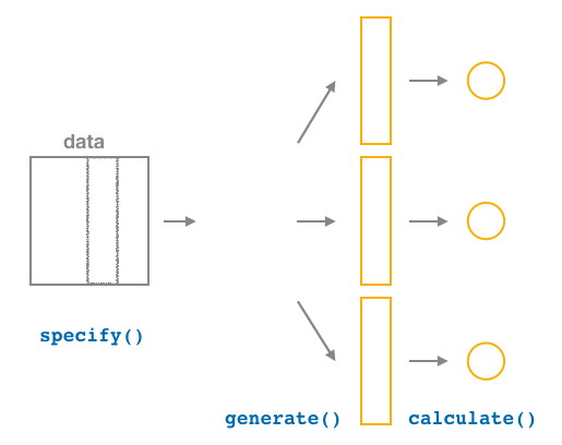
FIGURE 8.17: Diagram of calculate() summary statistics.
After we generate() 1000 bootstrap samples, we want to summarize each of them, for example, by calculating the sample mean of each one of them. As Figure 8.17 shows, the calculate() function does this.
In our example, we calculate the mean weight for each bootstrap sample by setting the stat argument equal to "mean" inside the calculate() function. The stat argument can be used for other common summary statistics such as "median", "sum", "sd" (standard deviation), and "prop" (proportion). To see a list of other possible summary statistics you can use, type ?calculate and read the help file.
Let’s save the result in a data frame called bootstrap_means and explore its contents:
bootstrap_means <- almonds_sample_100 |>
  specify(response = weight) |>
  generate(reps = 1000) |>
  calculate(stat = "mean")
Setting `type = "bootstrap"` in `generate()`.
bootstrap_meansResponse: weight (numeric)
# A tibble: 1,000 × 2
replicate stat
<int> <dbl>
1 1 3.68
2 2 3.688
3 3 3.632
4 4 3.68
5 5 3.679
6 6 3.675
7 7 3.678
8 8 3.706
9 9 3.643
10 10 3.68
# ℹ 990 more rowsObserve that the resulting data frame has 1000 rows and 2 columns corresponding to the 1000 replicate values. It also has the mean weight for each bootstrap sample saved in the variable stat.
Comparing with original workflow: You may have recognized at this point that the calculate() step in the infer workflow produces the same output as the summarize() step in the original workflow.
4. visualize the results
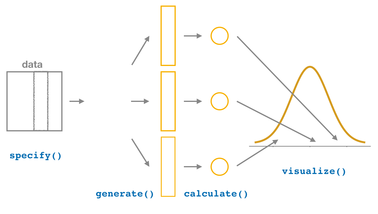
FIGURE 8.18: Diagram of visualize() results.
The visualize() verb provides a quick way to visualize the bootstrap distribution as a histogram of the numerical stat variable’s values as shown in Figure 8.19. The pipeline of the main infer verbs used for exploring bootstrap distribution results is shown in Figure 8.18.
visualize(bootstrap_means)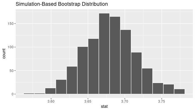
FIGURE 8.19: Bootstrap distribution.
Comparing with original workflow: In fact, visualize() is a wrapper function for the ggplot() function that uses a geom_histogram() layer. Recall that we illustrated the concept of a wrapper function in Figure 5.5 in Subsection 5.1.2.
# infer workflow:                    # Original workflow:
visualize(bootstrap_means)           ggplot(bootstrap_means, aes(x = stat)) +
                                        geom_histogram()
The visualize() function can take many other arguments to customize the plot further. In later sections, we take advantage of this flexibility. In addition, it works with helper functions to add shading of the histogram values corresponding to the confidence interval values.
We have introduced the different elements of the infer workflow for constructing a bootstrap distribution and visualizing it. A summary of these steps is presented in Figure 8.20.
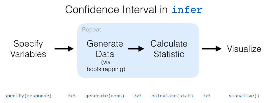
FIGURE 8.20: infer package workflow for confidence intervals.
8.2.4 Confidence intervals using bootstrap samples with infer
We are ready to introduce confidence intervals using the bootstrap via infer. We present two different methods for constructing 95% confidence intervals as interval estimates of an unknown population parameter: the percentile method and the standard error method{Bootstrap!standard error method}. Let’s now check out the infer package code that explicitly constructs these. There are also some additional neat functions to visualize the resulting confidence intervals built-in to the infer package.
Percentile method
Recall that in Subsection 8.2.3 we have generated 1000 bootstrap samples and stored them in data frame bootstrap_means:
bootstrap_meansResponse: weight (numeric)
# A tibble: 1,000 × 2
replicate stat
<int> <dbl>
1 1 3.68
2 2 3.688
3 3 3.632
4 4 3.68
5 5 3.679
6 6 3.675
7 7 3.678
8 8 3.706
9 9 3.643
10 10 3.68
# ℹ 990 more rowsThe sample means stored in bootstrap_means represent a good approximation to the bootstrap distribution of all possible bootstrap samples. The percentile method for constructing 95% confidence intervals sets the lower endpoint of the confidence interval at the 2.5th percentile of bootstrap_means and similarly sets the upper endpoint at the 97.5th percentile. The resulting interval captures the middle 95% of the values of the sample mean weights of almonds in bootstrap_means. This is the interval estimate of the population mean weight of almonds in the entire bowl.
We can compute the 95% confidence interval by piping bootstrap_means into the get_confidence_interval() function from the infer package, with the confidence level set to 0.95 and the confidence interval type to be "percentile". We save the results in percentile_ci.
percentile_ci <- bootstrap_means |>
  get_confidence_interval(level = 0.95, type = "percentile")
percentile_ci
# A tibble: 1 × 2
lower_ci upper_ci
<dbl> <dbl>
1 3.61198 3.756Alternatively, we can visualize the interval (3.61, 3.76) by piping the bootstrap_means data frame into the visualize() function and adding a shade_confidence_interval() layer. We set the endpoints argument to be percentile_ci.
visualize(bootstrap_means) +
  shade_confidence_interval(endpoints = percentile_ci)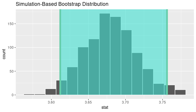
FIGURE 8.21: Percentile method 95% confidence interval shaded corresponding to potential values.
Observe in Figure 8.21 that 95% of the sample means stored in the stat variable in bootstrap_means fall between the two endpoints marked with the darker lines, with 2.5% of the sample means to the left of the shaded area and 2.5% of the sample means to the right. You also have the option to change the colors of the shading using the color and fill arguments.
The infer package has incorporated a shorter named function shade_ci() that produces the same results. Try out the following code:
Standard error method
In Subsection 8.1.3 we introduced theory-based confidence intervals. We show that a 95% confidence interval can be constructed as
\[\left(\overline{x} - 1.96 \cdot SE(\bar x), \quad \overline{x} + 1.96 \cdot SE(\bar x)\right)\]
where \(\overline{x}\) is the sample mean of the original sample, 1.96 is the number of standard errors around the mean needed to account for 95% of the area under the density curve (when the distribution is normal), and \(SE(\bar x)\) is the standard error of the sample mean that can be computed as \(\sigma /\sqrt{n}\) if the population standard deviation is known, or estimated as \(s/\sqrt{n}\) if we have to use the sample standard deviation, \(s\), and the sample size, \(n\).
We use the same structure to construct confidence intervals but using the bootstrap sample means to estimate the standard error of \(\overline{x}\). Thus, the 95% confidence interval for the population mean, \(\mu\), using the standard error estimated via bootstrapping, \(SE_\text{boot}\), is:
\[\left(\overline{x} - 1.96 \cdot SE_{\text{boot}}, \quad \overline{x} + 1.96 \cdot SE_{\text{boot}}\right)\]
We can compute this confidence interval using dplyr. First, we calculate the estimated standard error:
[1] 0.0357and then use the original sample mean to calculate the 95% confidence interval:
almonds_sample_100 |>
  summarize(lower_bound = mean(weight) - 1.96 * SE_boot,
            upper_bound = mean(weight) + 1.96 * SE_boot)
# A tibble: 1 × 2
lower_bound upper_bound
<dbl> <dbl>
1 3.61210 3.75190Alternatively, computation of the 95% confidence interval can once again be done via infer. We find the sample mean of the original sample and store it in variable x_bar
Response: weight (numeric)
# A tibble: 1 × 1
   stat
  <dbl>
1 3.682
Now, we pipe the bootstrap_means data frame we created into the get_confidence_interval() function. We set the type argument to be "se" and specify the point_estimate argument to be x_bar in order to set the center of the confidence interval to the sample mean of the original sample.
standard_error_ci <- bootstrap_means |>
  get_confidence_interval(type = "se", point_estimate = x_bar, level = 0.95)
standard_error_ci
# A tibble: 1 × 2
lower_ci upper_ci
<dbl> <dbl>
1 3.61210 3.75190The results are the same whether dplyr or infer is used, but as explained earlier, the latter provides more flexibility for other tests.
If we would like to visualize the interval (3.61, 3.75), we can once again pipe the bootstrap_means data frame into the visualize() function and add a shade_confidence_interval() layer to our plot. We set the endpoints argument to be standard_error_ci. The resulting standard-error method based on a 95% confidence interval for \(\mu\) can be seen in Figure 8.22.
visualize(bootstrap_means) +
  shade_confidence_interval(endpoints = standard_error_ci)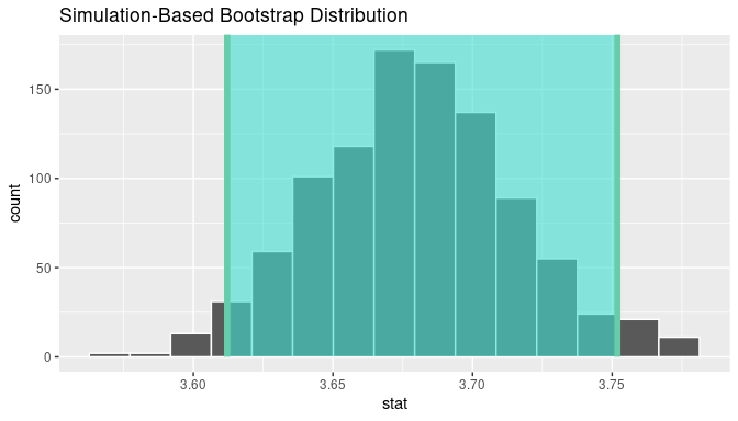
FIGURE 8.22: Standard-error method 95% confidence interval.
Because we are using bootstrap samples to construct these intervals, we call the percentile and standard error methods simulation-based methods. We can compare the 95% confidence intervals from using both simulation-based methods as well as the one attained using the theory-based method described in 8.1.3:
- Percentile method: (3.61, 3.76)
- Standard error method: (3.61, 3.75)
- Theory-based method: (3.61, 3.76)
Learning check
(LC8.14) Construct a 95% confidence interval for the median weight of all almonds with the percentile method. Is it appropriate to also use the standard-error method?
(LC8.15) What are the advantages of using infer for building confidence intervals?
(LC8.16) What is the main purpose of bootstrapping in statistical inference?
- A. To visualize data distributions and identify outliers.
- B. To generate multiple samples from the original data for estimating parameters.
- C. To replace missing data points with the mean of the dataset.
- D. To validate the assumptions of a regression model.
(LC8.17) “Which function denotes the variables of interest for inference?”
- A.
rep_sample_n() - B.
calculate() - C.
specify() - D.
visualize()
(LC8.18) What is a key difference between the percentile method and the standard error method for constructing confidence intervals using bootstrap samples?
- A. The percentile method requires the population standard deviation.
- B. The percentile method uses the middle 95% of bootstrap statistics, while the standard error method relies on the estimated standard error.
- C. The standard error method always results in a narrower confidence interval.
- D. The percentile method requires more bootstrap samples.
8.3 Additional remarks about the bootstrap
This section expands explanations on the bootstrap methods, provides some historical context, gives a comparison between the theory-based approach and the simulation-based approach when working with confidence intervals, and provides reasons for using the bootstrap. The presentation is more theoretical than other sections in this chapter, and you are welcome to skip to Section 8.4 if you want to go over directly another application of the bootstrap methods in R. Additional theoretical explanations are available in the Appendices of the online version of the book.
8.3.1 The bootstrap and other resampling methods
The bootstrap is one of many resampling methods. Chernick and LaBudde noted that the bootstrap’s roots trace back to the development of similar techniques like permutations and the jackknife (Chernick and LaBudde 2011). The bootstrap was initially conceived as an approximation to another resampling method called the jackknife but quickly gained recognition for its broader applicability and efficiency. Since then, it has been shown in multiple contexts that the bootstrap performs at least as well as traditional methods in estimating standard errors, constructing confidence intervals, performing hypothesis testing, and many other statistical techniques.
Furthermore, since the 1980s (but even more in the last two decades), the use of simulations to compare advanced bootstrap methods against other techniques, such as cross-validation, further established its superiority in specific contexts, particularly when dealing with small sample sizes. The use of the bootstrap and bootstrap-related methods has become a cornerstone in modern statistical and data science practices.
In this section, we introduce additional details about the bootstrap, and explain the advantages and limitations of using the bootstrap.
8.3.2 Confidence intervals and rate of convergence
We want to compare how the bootstrap performs when building confidence intervals with respect to the theory-based approach discussed in Section 8.1. The formal comparison requires mathematical concepts beyond the scope of this book, and it is not pursued here. Instead, we provide just enough elements to help you with the intuition of how this comparison is made and why bootstrap-related methods can be as strong as or even stronger than theory-based or alternative methods.
Let’s start with an illustration using the theory-based confidence interval. A 95% confidence interval for \(\mu\), when a sample of size \(n = 100\) is used, is given by
\[\overline{x} \pm 1.96 \frac{\sigma}{\sqrt{n}}\]
when \(\sigma\) is unknown or
\[\overline{x} \pm 1.98 \frac{s}{\sqrt{n}}\]
when \(\sigma\) is unknown. We use 95% and \(n = 100\) for this illustration, but the exposition is also true with any other confidence level or other sample sizes. We understand that 95% of all the possible samples would lead to an interval that contains \(\mu\). This statement is exactly true if the distribution of \(\overline X\) is precisely normal, and we say that 95% is the true coverage probability. In reality, we do not know what is the distribution of the population, but because of the Central Limit Theorem we know that for a large sample size \(n\) the distribution of \(\overline X\) is approximately normal. In this case, the 95% is an approximate coverage probability. This means that if we were to take every possible sample of size \(n\) and construct a confidence interval using the formulas above, not exactly 95% of the intervals will include \(\mu\). Again, this happens because \(\overline X\) is not exactly, but approximately, normal. Still, the Central Limit Theorem states that when \(n\) tends to infinity, the distribution of \(\overline X\) tends to normal, so the larger the sample size \(n\) the closer the distribution of \(\overline X\) is to the normal distribution, and the smaller the difference between the true and the approximate coverage probability.
Given that we can never make \(n\) infinity in real-life applications, we would like to produce 95% confidence intervals that make the difference between the approximate coverage probability and the true coverage probability as small as possible when we increase the sample size of our sample. Imagine a sequence of sample sizes \(n_1, n_2, n_3,\dots\) that gets bigger and bigger and bigger. The rate at which the corresponding consecutive differences in confidence intervals’ coverage probability decreases is called the rate of convergence of the difference between approximate and true coverage probabilities.
In the case of a 95% confidence interval for \(\mu\) using the theory-based approach, the rate of convergence for the difference is about \(1/\sqrt{n}\). This means that if we increase \(n\) from 100 to 400, the difference between the approximate and true coverage goes down from a factor of \(1/\sqrt{100} = 0.1\) to a factor of \(1/\sqrt{400} = 0.05\). Thus, increasing \(n\) four times leads to a decrease of the difference of about two times. In the statistical literature, a method that has this rate of convergence is called a first-order correct (Hall 1992) or first-order accurate (Chernick and LaBudde 2011).
The bootstrap percentile method discussed in 8.2.4, in the case of a 95% confidence interval for \(\mu\), is also first-order accurate. Thus, confidence intervals calculated using the theory-based and the bootstrap percentile method are comparable. This is consistent with the results we obtained earlier in this chapter.
In general, if you have two different methods that produce similar 95% confidence intervals and we need to choose one of them, we would choose the one that has a faster rate of convergence. As we discuss in the next subsection, other bootstrap methods have, in certain contexts, faster rates of convergence.
8.3.3 Why bootstrap methods
Why is it suitable to learn and use bootstrap methods for confidence intervals? The most important reason is that bootstrap methods, in particular advanced bootstrap methods, can deal with many limitations of the theory-based approach. Let’s discuss three of these limitations.
First, a 95% confidence interval for \(\mu\) is appropriate if the population distribution is not too extreme and the sample size is large enough for the distribution of \(\overline X\) to be approximately normal. But there are situations where these conditions are not satisfied, for example, if the population distribution is heavily skewed to the right, as in the case of income or wealth; or the distribution is constructed from only two values (1 or 0) but the chances of getting zero are much greater than the ones of getting one (for example, chance of getting zero is 0.999 and chance of getting 1 is 0.001) as it is the case in lottery outcomes or the presence of some disease in a population. When these situations are present, the confidence intervals would be inaccurate because the sample mean \(\overline X\) is biased when \(n\) is not too large. This means that if you were to take a large number of random samples and construct the sample mean of these samples, their average will be clearly different than \(\mu\), breaking down the theory we developed in Subsection 8.1. This problem may be fixed if the sample size is large, but, depending on how extreme the population distribution is, the sample size may need to be extremely large; perhaps in the order of thousands, or tens of thousands, or even more. Getting samples of those sizes may not be doable in real-life situations.
Second, in this chapter, we have study confidence intervals for the population mean \(\mu\), because it is a fundamental quantity and it is the foundation for other cases. However, building confidence intervals for other parameters using the theory-based approach (for example, for the median, the first quartile, the standard deviation, etc.) becomes more complicated or even unfeasible.
Third, when working with estimators more complicated than \(\overline X\), it is often not possible to derive the standard error estimator with a formula as clean as \(\sigma/\sqrt{n}\). Sometimes, there is no formula for the standard error and alternative methods have to be used to estimate it. This can create an additional source of bias. When bias is present, the confidence intervals created using the theory-based approach in Subsection 8.1.3 could be suspect, even completely useless.
The bootstrap percentile method is not affected directly by the second and third limitations. It can be implemented for any other parameter beyond the population mean, as long as all the information needed can be extracted from each bootstrap sample. On the other hand, the first limitation listed above can also affect the accuracy of this method.
Fortunately, since the inception of the bootstrap, many improvements have been made to the percentile method. Bootstrap methods have been proposed that address the presence of bias either by the limitations discussed above or the bias created when obtaining estimators or incorporating these methods. In addition, in certain contexts, these methods also improve the rate of convergence of the difference between the approximate and true coverage probability. Some of these methods are the percentile-\(t\) and the Bias Correction and Acceleration bootstrap method (BCa). In terms of rates of convergence, these methods are second-order accurate; that is, they have a rate of convergence of about \(1/n\). Another method called the double bootstrap (or more generally, the iterated bootstrap) can even be a third-order accurate.
We have not included these methods directly here because the theory that
justifies them goes beyond the scope of this book and, when dealing with
confidence intervals for \(\mu\) from populations with distributions that are not
extreme, there are not real gains in using them over the theory-based approach
or the percentile method. (We encourage you to check out one implementation of
bias-corrected confidence intervals in the infer package by setting
type = "bias-corrected" in the get_confidence_interval()
function.)
To summarize, when working with skewed distributions, small sample sizes, estimators of parameters other than \(\mu\) (such as the median), or the estimation of the standard error when there are no formulas to obtain them, many advanced bootstrap methods would be preferred over the theory-based approach. In the Appendices of the online version of the book, we plan to explore some of these advanced methods and present simulations that show when these methods are preferred over the percentile method or the theory-based approach.
8.4 Case study: is yawning contagious?
Let’s apply our knowledge of confidence intervals to answer the question: “Is yawning contagious?”. If you see someone else yawn, are you more likely to yawn? In an episode of the US show Mythbusters that aired on Discovery, the hosts conducted an experiment to answer this question. More information about the episode is available on IMDb.
8.4.1 Mythbusters study data
Fifty adult participants who thought they were being considered for an appearance on the show were interviewed by a show recruiter. In the interview, the recruiter either yawned or did not. Participants then sat by themselves in a large van and were asked to wait. While in the van, the Mythbusters team watched the participants using a hidden camera to see if they yawned. The data frame containing the results of their experiment is available as mythbusters_yawn included in the moderndive package:
mythbusters_yawn# A tibble: 50 × 3
subj group yawn
<int> <chr> <chr>
1 1 seed yes
2 2 control yes
3 3 seed no
4 4 seed yes
5 5 seed no
6 6 control no
7 7 seed yes
8 8 control no
9 9 control no
10 10 seed no
# ℹ 40 more rowsThe variables are:
-
subj: The participant ID with values 1 through 50. -
group: A binary treatment variable indicating whether the participant was exposed to yawning."seed"indicates the participant was exposed to yawning while"control"indicates the participant was not. -
yawn: A binary response variable indicating whether the participant ultimately yawned.
Recall that you learned about treatment and response variables in Subsection 5.3.1 in our discussion on confounding variables.
Let’s use some data wrangling to calculate counts of the four possible outcomes:
# A tibble: 4 × 3
# Groups:   group, yawn [4]
  group   yawn  count
  <chr>   <chr> <int>
1 control no       12
2 control yes       4
3 seed    no       24
4 seed    yes      10
Let’s first focus on the "control" group participants who were not exposed to yawning. 12 such participants did not yawn, while 4 such participants did. So out of the 16 people who were not exposed to yawning, 4/16 = 0.25 = 25% did yawn.
Let’s now focus on the "seed" group participants who were exposed to yawning where 24 such participants did not yawn, while 10 such participants did yawn. So out of the 34 people who were exposed to yawning, 10/34 = 0.294 = 29.4% did yawn. Comparing these two percentages, the participants who were exposed to yawning yawned 29.4% - 25% = 4.4% more often than those who were not.
8.4.2 Sampling scenario
Let’s review the terminology and notation related to sampling we studied in Subsection 7.2.1. In Chapter 7, our study population was the bowl of \(N\) = 2400 balls. Our population parameter of interest was the population proportion of these balls that were red, denoted mathematically by \(p\). In order to estimate \(p\), we extracted a sample of 50 balls using the shovel and computed the relevant point estimate: the sample proportion that were red, denoted mathematically by \(\widehat{p}\).
Who is the study population here? All humans? All the people who watch the show Mythbusters? It’s hard to say! This question can only be answered if we know how the show’s hosts recruited participants! In other words, what was the sampling methodology used by the Mythbusters to recruit participants? We alas are not provided with this information. Only for the purposes of this case study, however, we’ll assume that the 50 participants are a representative sample of all Americans given the popularity of this show. Thus, we’ll be assuming that any results of this experiment will generalize to all \(N\) = 346 million Americans (2024 population estimate).
Just like with our sampling bowl, the population parameter here will involve proportions. However, in this case, it will be the difference in population proportions \(p_{seed} - p_{control}\), where \(p_{seed}\) is the proportion of all Americans who if exposed to yawning will yawn themselves, and \(p_{control}\) is the proportion of all Americans who if not exposed to yawning still yawn themselves. Correspondingly, the point estimate/sample statistic based on the Mythbusters’ sample of participants will be the difference in sample proportions \(\widehat{p}_{seed} - \widehat{p}_{control}\). Let’s extend Table 8.1 of scenarios of sampling for inference to include our latest scenario.
| Scenario | Population parameter | Notation | Point estimate | Symbol(s) |
|---|---|---|---|---|
| 1 | Population proportion | \(p\) | Sample proportion | \(\widehat{p}\) |
| 2 | Population mean | \(\mu\) | Sample mean | \(\overline{x}\) or \(\widehat{\mu}\) |
| 3 | Difference in population proportions | \(p_1 - p_2\) | Difference in sample proportions | \(\widehat{p}_1 - \widehat{p}_2\) |
This is known as a two-sample inference situation since we have two separate samples. Based on their two-samples of size \(n_{seed}\) = 34 and \(n_{control}\) = 16, the point estimate is
\[ \widehat{p}_{seed} - \widehat{p}_{control} = \frac{24}{34} - \frac{12}{16} = 0.04411765 \approx 4.4\% \]
However, say the Mythbusters repeated this experiment. In other words, say they recruited 50 new participants and exposed 34 of them to yawning and 16 not. Would they find the exact same estimated difference of 4.4%? Probably not, again, because of sampling variation.
How does this sampling variation affect their estimate of 4.4%? In other words, what would be a plausible range of values for this difference that accounts for this sampling variation? We can answer this question with confidence intervals! Furthermore, since the Mythbusters only have a single two-sample of 50 participants, they would have to construct a 95% confidence interval for \(p_{seed} - p_{control}\) using bootstrap resampling with replacement.
We make a couple of important notes. First, for the comparison between the "seed" and "control" groups to make sense, however, both groups need to be independent from each other. Otherwise, they could influence each other’s results. This means that a participant being selected for the "seed" or "control" group has no influence on another participant being assigned to one of the two groups. As an example, if there were a mother and her child as participants in the study, they wouldn’t necessarily be in the same group. They would each be assigned randomly to one of the two groups of the explanatory variable.
Second, the order of the subtraction in the difference doesn’t matter so long as you are consistent and tailor your interpretations accordingly. In other words, using a point estimate of \(\widehat{p}_{seed} - \widehat{p}_{control}\) or \(\widehat{p}_{control} - \widehat{p}_{seed}\) does not make a material difference, you just need to stay consistent and interpret your results accordingly.
8.4.3 Constructing the confidence interval
As we did in Subsection 8.2.3, let’s first construct the bootstrap distribution for \(\widehat{p}_{seed} - \widehat{p}_{control}\) and then use this to construct 95% confidence intervals for \(p_{seed} - p_{control}\). We’ll do this using the infer workflow again. However, since the difference in proportions is a new scenario for inference, we’ll need to use some new arguments in the infer functions along the way.
1. specify variables
Let’s take our mythbusters_yawn data frame and specify() which variables are of interest using the y ~ x formula interface where:
- Our response variable is
yawn: whether or not a participant yawned. It has levels"yes"and"no". - The explanatory variable is
group. It has levels"seed"(exposed to yawning) and"control"(not exposed to yawning).
mythbusters_yawn |>
  specify(formula = yawn ~ group)
Error: A level of the response variable `yawn` needs to be specified for the
`success` argument in `specify()`.Alas, we got an error message that infer is telling us that one of the levels of the categorical variable yawn needs to be defined as the success. Recall that we define success to be the event of interest we are trying to count and compute proportions of. Are we interested in those participants who "yes" yawned or those who "no" didn’t yawn? This isn’t clear to R or someone just picking up the code and results for the first time, so we need to set the success argument to "yes" as follows to improve the transparency of the code:
mythbusters_yawn |>
  specify(formula = yawn ~ group, success = "yes")
Response: yawn (factor)
Explanatory: group (factor)
# A tibble: 50 × 2
yawn group
<fct> <fct>
1 yes seed
2 yes control
3 no seed
4 yes seed
5 no seed
6 no control
7 yes seed
8 no control
9 no control
10 no seed
# ℹ 40 more rows2. generate replicates
Our next step is to perform bootstrap resampling with replacement like we did with the almonds in the activity in Section 8.2.1. We saw how it works with both a single variable in computing bootstrap means in Section 8.2.2, but we haven’t yet worked with bootstrapping involving multiple variables.
In the infer package, bootstrapping with multiple variables means that each row is potentially resampled. Let’s investigate this by focusing only on the first six rows of mythbusters_yawn:
first_six_rows <- head(mythbusters_yawn)
first_six_rows
# A tibble: 6 × 3
subj group yawn
<int> <chr> <chr>
1 1 seed yes
2 2 control yes
3 3 seed no
4 4 seed yes
5 5 seed no
6 6 control no When we bootstrap this data, we are potentially pulling the subject’s readings multiple times. Thus, we could see the entries of "seed" for group and "no" for yawn together in a new row in a bootstrap sample. This is further seen by exploring the sample_n() function in dplyr on this smaller 6-row data frame comprised of head(mythbusters_yawn). The sample_n() function can perform this bootstrapping procedure and is similar to the rep_sample_n() function in infer, except that it is not repeated, but rather only performs one sample with or without replacement.
first_six_rows |>
  sample_n(size = 6, replace = TRUE)
# A tibble: 6 × 3
subj group yawn
<int> <chr> <chr>
1 6 control no
2 1 seed yes
3 2 control yes
4 6 control no
5 4 seed yes
6 4 seed yes We can see that in this bootstrap sample generated from the first six rows of mythbusters_yawn, we have some rows repeated. The same is true when we perform the generate() step in infer as done in what follows. Using this fact, we generate 1000 replicates, or, in other words, we bootstrap resample the 50 participants with replacement 1000 times.
mythbusters_yawn |>
  specify(formula = yawn ~ group, success = "yes") |>
  generate(reps = 1000, type = "bootstrap")
Response: yawn (factor)
Explanatory: group (factor)
# A tibble: 50,000 × 3
# Groups: replicate [1,000]
replicate yawn group
<int> <fct> <fct>
1 1 yes seed
2 1 yes control
3 1 no control
4 1 no control
5 1 yes seed
6 1 yes seed
7 1 yes seed
8 1 yes seed
9 1 no seed
10 1 yes seed
# ℹ 49,990 more rowsObserve that the resulting data frame has 50,000 rows. This is because we performed resampling of 50 participants with replacement 1000 times and 50,000 = 1000 \(\cdot\) 50. The variable replicate indicates which resample each row belongs to. So it has the value 1 50 times, the value 2 50 times, all the way through to the value 1000 50 times.
3. calculate summary statistics
After we generate() many replicates of bootstrap resampling with replacement, we next want to summarize the bootstrap resamples of size 50 with a single summary statistic, the difference in proportions. We do this by setting the stat argument to "diff in props":
mythbusters_yawn |>
  specify(formula = yawn ~ group, success = "yes") |>
  generate(reps = 1000, type = "bootstrap") |>
  calculate(stat = "diff in props")
Warning message:
The statistic is based on a difference or ratio; by default, for
difference-based statistics, the explanatory variable is subtracted in the
order "control" - "seed", or divided in the order "control" / "seed" for
ratio-based statistics. To specify this order yourself, supply
`order = c("control", "seed")` to the calculate() function. We see another warning here. We need to specify the order of the subtraction. Is it \(\widehat{p}_{seed} - \widehat{p}_{control}\) or \(\widehat{p}_{control} - \widehat{p}_{seed}\). We specify it to be \(\widehat{p}_{seed} - \widehat{p}_{control}\) by setting order = c("seed", "control"). Note that you could’ve also set order = c("control", "seed"). As we stated earlier, the order of the subtraction does not matter, so long as you stay consistent throughout your analysis and tailor your interpretations accordingly.
Let’s save the output in a data frame bootstrap_distribution_yawning:
bootstrap_distribution_yawning <- mythbusters_yawn |>
  specify(formula = yawn ~ group, success = "yes") |>
  generate(reps = 1000, type = "bootstrap") |>
  calculate(stat = "diff in props", order = c("seed", "control"))
bootstrap_distribution_yawning
# A tibble: 1,000 × 2
replicate stat
<int> <dbl>
1 1 0.0357143
2 2 0.229167
3 3 0.00952381
4 4 0.0106952
5 5 0.00483092
6 6 0.00793651
7 7 -0.0845588
8 8 -0.00466200
9 9 0.164686
10 10 0.124777
# ℹ 990 more rowsObserve that the resulting data frame has 1000 rows and 2 columns corresponding to the 1000 replicate ID’s and the 1000 differences in proportions for each bootstrap resample in stat.
4. visualize the results
In Figure 8.23 we visualize() the resulting bootstrap resampling distribution. Let’s also add a vertical line at 0 by adding a geom_vline() layer.
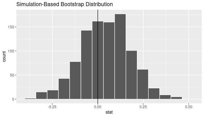
FIGURE 8.23: Bootstrap distribution.
First, let’s compute the 95% confidence interval for \(p_{seed} - p_{control}\) using the percentile method, in other words, by identifying the 2.5th and 97.5th percentiles which include the middle 95% of values. Recall that this method does not require the bootstrap distribution to be normally shaped.
bootstrap_distribution_yawning |>
  get_confidence_interval(type = "percentile", level = 0.95)
# A tibble: 1 × 2
lower_ci upper_ci
<dbl> <dbl>
1 -0.238276 0.302464Second, since the bootstrap distribution is roughly bell-shaped, we can construct a confidence interval using the standard error method as well. Recall that to construct a confidence interval using the standard error method, we need to specify the center of the interval using the point_estimate argument. In our case, we need to set it to be the difference in sample proportions of 4.4% that the Mythbusters observed.
We can also use the infer workflow to compute this value by excluding the generate() 1000 bootstrap replicates step. In other words, do not generate replicates, but rather use only the original sample data. We can achieve this by commenting out the generate() line, telling R to ignore it:
obs_diff_in_props <- mythbusters_yawn |>
  specify(formula = yawn ~ group, success = "yes") |>
  # generate(reps = 1000, type = "bootstrap") |>
  calculate(stat = "diff in props", order = c("seed", "control"))
obs_diff_in_props
Response: yawn (factor)
Explanatory: group (factor)
# A tibble: 1 × 1
stat
<dbl>
1 0.0441176We thus plug this value in as the point_estimate argument.
myth_ci_se <- bootstrap_distribution_yawning |>
  get_confidence_interval(type = "se", point_estimate = obs_diff_in_props,
                          level = 0.95)
myth_ci_se
# A tibble: 1 × 2
lower_ci upper_ci
<dbl> <dbl>
1 -0.227291 0.315526Let’s visualize both confidence intervals in Figure 8.24, with the percentile method interval marked with black lines and the standard-error method marked with grey lines. Observe that they are both similar to each other.
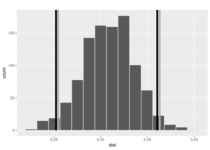
FIGURE 8.24: Two 95% confidence intervals: percentile method (black) and standard error method (grey).
8.4.4 Interpreting the confidence interval
Given that both confidence intervals are quite similar, let’s focus our interpretation to only the percentile method confidence interval of (-0.238, 0.302). The precise statistical interpretation of a 95% confidence interval is: if this construction procedure is repeated 100 times, then we expect about 95 of the confidence intervals to capture the true value of \(p_{seed} - p_{control}\). In other words, if we gathered 100 samples of \(n\) = 50 participants from a similar pool of people and constructed 100 confidence intervals each based on each of the 100 samples, about 95 of them will contain the true value of \(p_{seed} - p_{control}\) while about five won’t. Given that this is a little long winded, we use the shorthand interpretation: we’re 95% “confident” that the true difference in proportions \(p_{seed} - p_{control}\) is between (-0.238, 0.302).
There is one value of particular interest that this 95% confidence interval contains: zero. If \(p_{seed} - p_{control}\) were equal to 0, then there would be no difference in proportion yawning between the two groups. This would suggest that there is no associated effect of being exposed to a yawning recruiter on whether you yawn yourself.
In our case, since the 95% confidence interval includes 0, we cannot conclusively say if either proportion is larger. Of our 1000 bootstrap resamples with replacement, sometimes \(\widehat{p}_{seed}\) was higher and thus those exposed to yawning yawned themselves more often. At other times, the reverse happened.
Say, on the other hand, the 95% confidence interval was entirely above zero. This would suggest that \(p_{seed} - p_{control} > 0\), or, in other words \(p_{seed} > p_{control}\), and thus we’d have evidence suggesting those exposed to yawning do yawn more often.
8.5 Summary and final remarks
8.5.1 Additional resources
If you want more examples of the infer workflow to construct confidence intervals, we suggest you check out the infer package homepage, in particular, a series of example analyses available at https://infer.netlify.app/articles/.
8.5.2 What’s to come?
Now that we’ve equipped ourselves with confidence intervals, in Chapter 9 we’ll cover the other common tool for statistical inference: hypothesis testing. Just like confidence intervals, hypothesis tests are used to infer about a population using a sample. However, we’ll see that the framework for making such inferences is slightly different.