A Statistical Background

A.1 Basic statistical terms

Note that all the following statistical terms apply only to numerical variables, except the distribution which can exist for both numerical and categorical variables.

A.1.1 Mean

The mean is the most commonly reported measure of center. It is commonly called the average though this term can be a little ambiguous. The mean is the sum of all of the data elements divided by how many elements there are. If we have $n$ data points, the mean is given by:

\[Mean = \frac{x_1 + x_2 + \cdots + x_n}{n}\]

A.1.2 Median

The median is calculated by first sorting a variable’s data from smallest to largest. After sorting the data, the middle element in the list is the median. If the middle falls between two values, then the median is the mean of those two middle values.

A.1.3 Standard deviation and variance

We will next discuss the standard deviation ($sd$) of a variable. The formula can be a little intimidating at first but it is important to remember that it is essentially a measure of how far we expect a given data value will be from its mean:

\[sd = \sqrt{\frac{(x_1 - Mean)^2 + (x_2 - Mean)^2 + \cdots + (x_n - Mean)^2}{n - 1}}\]

The variance of a variable is merely the standard deviation squared.

\[variance = sd^2 = \frac{(x_1 - Mean)^2 + (x_2 - Mean)^2 + \cdots + (x_n - Mean)^2}{n - 1}\]

A.1.4 Five-number summary

The five-number summary consists of five summary statistics: the minimum, the first quantile AKA 25th percentile, the second quantile AKA median or 50th percentile, the third quantile AKA 75th, and the maximum. The five-number summary of a variable is used when constructing boxplots, as seen in Section 2.7.

The quantiles are calculated as

first quantile ($Q_1$): the median of the first half of the sorted data
third quantile ($Q_3$): the median of the second half of the sorted data

The interquartile range (IQR) is defined as $Q_3 - Q_1$ and is a measure of how spread out the middle 50% of values are. The IQR corresponds to the length of the box in a boxplot.

The median and the IQR are not influenced by the presence of outliers in the ways that the mean and standard deviation are. They are, thus, recommended for skewed datasets. We say in this case that the median and IQR are more robust to outliers.

A.1.5 Distribution

The distribution of a variable shows how frequently different values of a variable occur. Looking at the visualization of a distribution can show where the values are centered, show how the values vary, and give some information about where a typical value might fall. It can also alert you to the presence of outliers.

Recall from Chapter 2 that we can visualize the distribution of a numerical variable using binning in a histogram and that we can visualize the distribution of a categorical variable using a barplot.

A.1.6 Outliers

Outliers correspond to values in the dataset that fall far outside the range of “ordinary” values. In the context of a boxplot, by default they correspond to values below $Q_1 - (1.5 \cdot IQR)$ or above $Q_3 + (1.5 \cdot IQR)$.

A.2 Normal distribution

Let’s next discuss one particular kind of distribution: normal distributions. Such bell-shaped distributions are defined by two values: (1) the mean $\mu$ (“mu”) which locates the center of the distribution and (2) the standard deviation $\sigma$ (“sigma”) which determines the variation of the distribution. In Figure A.1, we plot three normal distributions where:

The solid normal curve has mean $\mu = 5$ & standard deviation $\sigma = 2$.
The dotted normal curve has mean $\mu = 5$ & standard deviation $\sigma = 5$.
The dashed normal curve has mean $\mu = 15$ & standard deviation $\sigma = 2$.

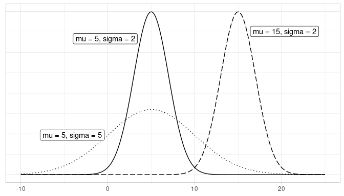
FIGURE A.1: Three normal distributions.

Notice how the solid and dotted line normal curves have the same center due to their common mean $\mu$ = 5. However, the dotted line normal curve is wider due to its larger standard deviation of $\sigma$ = 5. On the other hand, the solid and dashed line normal curves have the same variation due to their common standard deviation $\sigma$ = 2. However, they are centered at different locations.

When the mean $\mu$ = 0 and the standard deviation $\sigma$ = 1, the normal distribution has a special name. It’s called the standard normal distribution or the $z$-curve.

Furthermore, if a variable follows a normal curve, there are three rules of thumb we can use:

68% of values will lie within $\pm$ 1 standard deviation of the mean.
95% of values will lie within $\pm$ 1.96 $\approx$ 2 standard deviations of the mean.
99.7% of values will lie within $\pm$ 3 standard deviations of the mean.

Let’s illustrate this on a standard normal curve in Figure A.2. The dashed lines are at -3, -1.96, -1, 0, 1, 1.96, and 3. These 7 lines cut up the x-axis into 8 segments. The areas under the normal curve for each of the 8 segments are marked and add up to 100%. For example:

The middle two segments represent the interval -1 to 1. The shaded area above this interval represents 34% + 34% = 68% of the area under the curve. In other words, 68% of values.
The middle four segments represent the interval -1.96 to 1.96. The shaded area above this interval represents 13.5% + 34% + 34% + 13.5% = 95% of the area under the curve. In other words, 95% of values.
The middle six segments represent the interval -3 to 3. The shaded area above this interval represents 2.35% + 13.5% + 34% + 34% + 13.5% + 2.35% = 99.7% of the area under the curve. In other words, 99.7% of values.

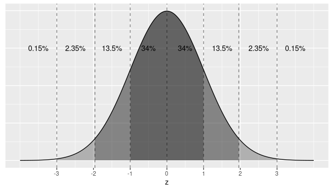
FIGURE A.2: Rules of thumb about areas under normal curves.

Learning check

Say you have a normal distribution with mean $\mu = 6$ and standard deviation $\sigma = 3$.

(LCA.1) What proportion of the area under the normal curve is less than 3? Greater than 12? Between 0 and 12?

(LCA.2) What is the 2.5th percentile of the area under the normal curve? The 97.5th percentile? The 100th percentile?

A.2.1 Additional normal calculations

For a normal density curve, the probabilities or areas for any given interval can be obtained using the R function pnorm(). Think of the p in the name as __p__robability or __p__ercentage as this function finds the area under the curve to the left of any given value which is the probability of observing any number less than or equal to that value. It is possible to indicate the appropriate expected value and standard deviation as arguments in the function, but the default uses the standard normal values, $\mu = 0$ and $\sigma = 1$. For example, the probability of observing a value that is less than or equal to 1 in the standard normal curve is given by:

pnorm(1)

[1] 0.841

or 84%. This is the probability of observing a value that is less than or equal to one standard deviation above the mean.

Similarly, the probability of observing a standard value between -1 and 1 is given by subtracting the area to the left of -1 from the area to the left of 1. In R, we obtain this probability as follows:

pnorm(1) - pnorm(-1)

[1] 0.683

The probability of getting a standard value between -1 and 1, or equivalently, the probability of observing a value within one standard deviation from the mean is about 68%. Similarly, the probability of getting a value within 2 standard deviations from the mean is given by

pnorm(2) - pnorm(-2)

[1] 0.954

or about 95%.

Moreover, we do not need to restrict our study to areas within one or two standard deviations from the mean. We can find the number of standard deviations needed for any desired percentage around the mean using the R function qnorm(). The q in the name stands for $quantile$ and this function can be thought of as the inverse or complement of pnorm(). It finds the value of the random variable for a given area under the curve to the left of this value. When using the standard normal, the quantile also represents the number of standard deviations. For example, we learned that the area under the standard normal curve to the left of a standard value of 1 was approximately 84%. If instead, we want to find the standard value that corresponds to exactly an area of 84% under the curve to the left of this value, we can use the following syntax:

qnorm(0.84)

[1] 0.994

In other words, there is exactly an 84% chance that the observed standard value is less than or equal to 0.994. Similarly, to have exactly a 95% chance of obtaining a value within q number of standard deviations from the mean, we need to select the appropriate value for qnorm().

ggplot(NULL, aes(c(-4,4))) +
  geom_area(stat = "function", fun = dnorm, fill = "grey100", xlim = c(-4, -2)) +
  geom_area(stat = "function", fun = dnorm, fill = "grey80", xlim = c(-2, 2)) +
  geom_area(stat = "function", fun = dnorm, fill = "grey100", xlim = c(2, 4)) +
  labs(x = "z", y = "") +
  scale_y_continuous(breaks = NULL) +
  scale_x_continuous(breaks = NULL) + 
  annotate(geom="text", x=2, y=-0.01, label="q",
           color="blue")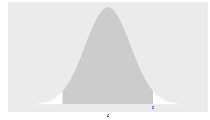

We want to find the standard value q such that the area in the middle is exactly 0.95 (or 95%). Before using qnorm() we need to provide the total area under the curve to the left of q. Since the total area under the normal density curve is 1, the curve is symmetric, and the area in the middle is 0.95, the total area on the tails is 1 - 0.95 = 0.05 (or 5%), and the area on each tail is 0.05/2 = 0.025 (or 2.5%). The total area under the curve to the left of q will be the area in the middle and the area on the left tail or 0.95 + 0.025 = 0.975. We can now obtain the standard value q by using qnorm():

q <- qnorm(0.975)
q

[1] 1.96

The probability of observing a value within 1.96 standard deviations from the mean is exactly 95%.

We can follow this method to obtain the number of standard deviations needed for any area, or probability, around the mean. For example, if we want an area of 98% around the mean, the area on the tails is 1 - 0.98 = 0.02, or 0.02/2 = 0.01 on each tail, the area under the curve to the left of the desired q value would be 0.98 + 0.01 = 0.99 so

qnorm(0.99)

[1] 2.33

The area within 2.33 standard deviations from the mean is 98%, or there is a 98% chance of choosing a value within 2.33 standard deviations from the mean. This information will be very useful to us.

A.3 The t distribution calculations

The syntax in R for the $t$ distribution is analogous to the standard normal distribution. We use the function pt() instead of pnorm() and qt() instead of qnorm(). In addition, the $t$ distribution requires one additional parameter, the degrees of freedom. For the sample mean problems, the degrees of freedom needed are exactly $n-1$, the size of the samples minus one.

We construct again a 95% confidence interval for the population mean, but this time using the sample standard deviation to estimate the standard error and the $t$ distribution to determine how wide the confidence interval should be.

We start by obtaining the sample statistics:

almonds_sample_100 |> 
summarize(mean_weight = mean(weight),
sd_weight = sd(weight),
sample_size = n())

# A tibble: 1 × 3
  mean_weight sd_weight sample_size
        <dbl>     <dbl>       <int>
1       3.682  0.362199         100

To obtain the number of standard deviations on the $t$ distribution to account for 95% of the values, we proceed as we did in the normal case: the area in the middle is 0.95, so the area on the tails is 1-0.95 = 0.05. Since the $t$ distribution is also symmetric, the area on each tail is 0.05/2 - 0.025. The number of standard deviation around the center is given by the value $q$ such as the area under the $t$ curve to the left of $q$ is exactly $0.95 + 0.025 = 0.975$. Using R we get:

qt(0.975, df = 100 - 1)

[1] 1.98

So, in order to account for 95% of the observations around the mean, we need to take into account all the values within 1.98 standard deviation from the mean. Compare this number with the 1.96 obtained for the standard normal; the difference is due to the fact that the $t$ curve has thicker tails than the standard normal. We can now construct the 95% confidence interval

xbar <- 3.682 
se_xbar <- 0.362/sqrt(100)
lower_bound <- xbar - 1.98 *  se_xbar
upper_bound <- xbar + 1.98 *  se_xbar
c(lower_bound, upper_bound)

[1] 3.61 3.75

We are 95% confident that the population mean weight of almonds is a number between 3.61 and 3.75 grams.

A.4 log10 transformations

At its simplest, log10 transformations return base 10 logarithms. For example, since $1000 = 10^3$, running log10(1000) returns 3 in R. To undo a log10 transformation, we raise 10 to this value. For example, to undo the previous log10 transformation and return the original value of 1000, we raise 10 to the power of 3 by running 10^(3) = 1000 in R.

Log transformations allow us to focus on changes in orders of magnitude. In other words, they allow us to focus on multiplicative changes instead of additive ones. Let’s illustrate this idea in Table A.1 with examples of prices of consumer goods in 2019 US dollars.

TABLE A.1: TABLE A.2: log10 transformed prices, orders of magnitude, and examples
Price	log10(Price)	Order of magnitude	Examples
$1	0	Singles	Cups of coffee
$10	1	Tens	Books
$100	2	Hundreds	Mobile phones
$1,000	3	Thousands	High definition TVs
$10,000	4	Tens of thousands	Cars
$100,000	5	Hundreds of thousands	Luxury cars and houses
$1,000,000	6	Millions	Luxury houses

Let’s make some remarks about log10 transformations based on Table A.1:

When purchasing a cup of coffee, we tend to think of prices ranging in single dollars, such as $2 or $3. However, when purchasing a mobile phone, we don’t tend to think of their prices in units of single dollars such as $313 or $727. Instead, we tend to think of their prices in units of hundreds of dollars like $300 or $700. Thus, cups of coffee and mobile phones are of different orders of magnitude in price.
Let’s say we want to know the log10 transformed value of $76. This would be hard to compute exactly without a calculator. However, since $76 is between $10 and $100 and since log10(10) = 1 and log10(100) = 2, we know log10(76) will be between 1 and 2. In fact, log10(76) is 1.880814.
log10 transformations are monotonic, meaning they preserve orders. So if Price A is lower than Price B, then log10(Price A) will also be lower than log10(Price B).
Most importantly, increments of one in log10-scale correspond to relative multiplicative changes in the original scale and not absolute additive changes. For example, increasing a log10(Price) from 3 to 4 corresponds to a multiplicative increase by a factor of 10: $100 to $1000.

11 Tell Your Story with Data

B Inference Examples